Download
1 / 45
460 likes | 614 Views
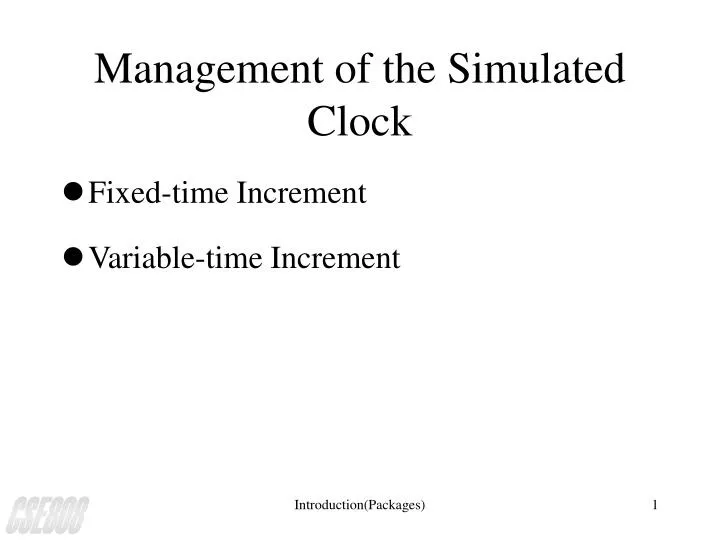
Management of the Simulated Clock. Fixed-time Increment Variable-time Increment. Arrival event. Schedule the next arrival event. Yes. Is the server busy?. No. Add 1to the number in queue. Set delay = 0 for this customer and gather statistics. Write error message and stop

E N D
Management of the Simulated Clock • Fixed-time Increment • Variable-time Increment Introduction(Packages)
Arrival event Schedule the next arrival event Yes Is the server busy? No Add 1to the number in queue Set delay = 0 for this customer and gather statistics Write error message and stop simulation Yes Is the queue Full? Add 1 to thenumber of customers delayed No Store time of arrival of this customer Make the server busy Schedule a departure event for this customer Return Flowchart for arrival routine, queueing model
Departure event Yes Is the queue empty? No Make the server idle Subtract 1 from the number in queue Eliminate departure event from consideration Compute delay of customer entering service and gather statistics Add 1 to the number of customers delayed Schedule a departure event for this customer Move each customer in queue (if any) up one place Return Flowchart for departure routine, queueing model
Time between Cumulative Random digit Arrivals(min.) Probability Probability Assignment 1 2 3 4 5 6 7 8 0.125 0.125 0.125 0.125 0.125 0.125 0.125 0.125 0.125 0.250 0.375 0.500 0.625 0.750 0.875 1.000 000-125 126-250 251-375 376-500 501-625 626-750 751-875 876-000 Distribution of time between arrivals Introduction(Packages)
Service Time Cumulative Random digit (Minutes) Probability Probability Assignment 1 0.10 0.10 01 - 10 2 0.20 0.30 11 - 30 3 0.30 0.60 31 - 60 4 0.25 0.85 61- 85 5 0.10 0.95 86 - 95 6 0.05 1.00 96 - 00 Service Time Distribution Introduction(Packages)
Random Time btwn Random Time btwn Digit Arrivals Digit Arrivals Customer (Minutes) Customer (Minutes) 1 _ _ 11 109 1 2 913 8 12 093 1 3 727 6 13 607 5 4 015 1 14 738 6 5 948 8 15 359 3 6 309 3 16 888 8 7 922 8 17 106 1 8 753 7 18 212 2 9 235 2 19 493 4 10 302 3 20 535 5 Time-between-arrival Determination Introduction(Packages)
Service Time (Minutes) Service Time (Minutes) Customer Random Digit Customer Random Digit 1 84 4 11 32 3 2 10 1 12 94 5 3 74 4 13 79 4 4 53 3 14 05 1 5 17 2 15 79 5 6 79 4 16 84 4 7 91 5 17 52 3 8 67 4 18 55 3 9 89 5 19 30 2 10 38 3 20 50 3 Service Times Generated Introduction(Packages)
Work Sheet Event Type Customer Number Clock Time Arrival 1 0 . . . . . . . . .
1. Average waiting time for a customer Total time customers wait in queue(minute) Total number of customers Findings from the Simulation Introduction(Packages)
2. Prob. that a customer has to wait in a queue Number of customers who wait Total number of customers Findings from the Simulation(cont) Introduction(Packages)
3. Proportion of idle time of the server Total idle time of server(minute) Total run time of simulation(minute) Thus, the probability of the server being busy is the complement of 0.21, or 0.79 Findings from the Simulation(cont) Introduction(Packages)
The Able-Baker carhop problem The purpose of this example is to indicate the simulation procedure when there is more than one channel. Consider a drive-in restaurant where carhops take orders and bring food to the car. Cars arrive in the manner shown in the following table. Introduction(Packages)
Time between Random Arrivals Cumulative Digit (Minutes) Probability Probability Assignment 1 0.25 0.25 01-25 2 0.40 0.65 26-65 3 0.20 0.85 66-85 4 0.15 1.00 86-00 The Able-Baker carhop problem(Interarrival distribution of cars) Introduction(Packages)
The Able-Baker carhop problem(continued) There are two car hops -- Able and Baker. Able is better able to do the job, and works somewhat faster than Baker. The distribution of service times of Able and Baker is following. Introduction(Packages)
Service Random Time Cumulative Digit (Minutes) Probability Probability Assignment 2 0.30 0.30 01-30 3 0.28 0.58 31-58 4 0.25 0.83 59-83 5 0.17 1.00 84-00 The Able-Baker carhop problem(Service Distribution of Able) Introduction(Packages)
Service Random Time Cumulative Digit (Minutes) Probability Probability Assignment 3 0.35 0.35 01-35 4 0.25 0.60 36-60 5 0.20 0.80 61-80 6 0.20 1.00 81-00 The Able-Baker carhop problem(Service Distribution of Baker) Introduction(Packages)
The Able-Baker carhop problem(Continued) • Over the 62-minute period Able is busy 90% of the time. • Baker was busy only 69% of the time. The seniority rule keeps Baker less busy. • Nine of 26 or about 35% of the arrivals had to wait. The average waiting time for all customers was only about 0.42 minute, or 25 seconds, which is very small. Introduction(Packages)
The Able-Baker carhop problem(Continued) • Those 9 who did have to wait only waited an average of 1.22 minutes, which is quite low. • In summary, this system seems well balanced. One server cannot handle all the dinners, and three servers would probably be too many. Adding an additional server would surely reduce the waiting time to nearly zero. However, the cost of waiting would have to be quite high to justify an additional worker. Introduction(Packages)
GPSS (Process-Oriented) Diagram Introduction(Packages)
GPSS Events • Current-Event Chain: Transaction with BDT <= C1 • Future-Event Chain: Transaction with BDT > C1 Introduction(Packages)
GPSS Events(continued) • Note Events must be executed chronologically, so chains are maintained in ascending order Current-Event Chain performs an additional tasks(i.e. maintains by priority) Introduction(Packages)
GPSS Execution Trace The system. Four transactions enter the system at intervals of 3 time units, starting at time unit 1. They try to seize facility MACH for 4 time units and then try to enter storage BUFFE (with capacity 2) before releasing MACH. After 9 time units in BUFFE, they leave storage and terminate. In this model the number of transactions must be limited because it has been devised to cause catastrophic congestion. Introduction(Packages)
GPSS Sample instructions BUFFE STORAGE 2 GENERATE 3,,1,4 QUEUE WAIT SEIZE MACH DEPART WAIT ADVANCE 4 ENTER BUFFE RELEASE MACH ADVANCE 9 LEAVE BUFFE TERMINATE 1 START 4 Introduction(Packages)
GPSS (Process-Oriented) Diagram Introduction(Packages)
GPSS/H Block Diagram, Queueing Model Introduction(Packages)
GPSS/H - Queueing Model 1 * SIMULATION OF THE M/M/1 QUEUE 2 * 3 SIMULATE 4 GENERATE RVEXPO(1,1,0) Create Arriving Customer 5 QUEUE SERVERQ Enter the Queue 6 SEIZE SERVER Seize the Server 7 LVEQ DEPART SERVERQ Leave the Queue 8 TEST L N$LVEQ,1000,STOP Test for Termination 9 ADVANCE RVEXPO(2,0.5) Delay for service 10 STOP RELEASE SERVER Customers Depart 11 TERMINATE 1 12 * 13 * CONTROL STATEMENT 14 * 15 START 1000 Make 1 simulation run 16 END Introduction(Packages)
GPSS/H standard output report, Queueing Model RELATIVE CLOCK: 1014.1565 ABSOLUTE CLOCK:1014.1565 BLOCK CURRENT TOTAL 1 1000 2 1000 3 1000 LVEQ 1000 5 1000 6 999 STOP 1000 8 1000 -- AVG-UTIL-DURING-- FACILITY TOTAL AVAIL UNAVL ENTRIES AVG CURRENT TIME TIME TIME TIME/XACT STATUS SERVER 0.516 1000 0.523 AVAIL Introduction(Packages)
GPSS/H standard output report, Queueing Model(Continued) QUEUE MAXIMUM AVERAGE TOTAL ZERO PERCENT CONTENTS CONTENTS ENTRIES ENTRIES ZEROS SERVERQ 8 0.605 1000 454 45.4 QUEUE AVERAGE $AVERAGE QTABLE CURRENT TIME/UNIT TIME/UNIT NUMBER CONTENTS SERVERQ 0.614 1.124 0 RANDOM ANTITHETIC INITIAL CURRENT SAMPLE CHI-SQUARE STREAM VARIATES POS. POS. COUNT UNIFORMITY 1 OFF 100000 101001 1001 0.71 2 OFF 200000 200999 999 0.69 Introduction(Packages)
SIMSCRIPT II.5 Preamble,Queueing Model 1 PREAMBLE 2 PROCESSES INCLUDE ARRIVAL.GENERATOR, 3 CUSTOMER, AND REPORT 4 RESOURCES INCLUDE SERVER 5 DEFINE DELAY.IN.QUEUE, MEAN.INTERARRIVAL.TIME, 6 AND MEAN.SERVICE.TIME AS REAL VARIABLES 7 DEFINE TOT.DELAYS AS AN INTEGER VARIABLE 8 DEFINE MINUTES TO MEAN UNITS 9 TALLY AVG.DELAY.IN.QUEUE AS THE AVERAGE AND 10 NUM.DELAYS AS THE NUMBER OF DELAY.IN.QUEUE 11 ACCUMULATE AVG.NUMBER.IN.QUEUE AS THE 12 AVERAGE OF N.Q.SERVER 13 ACCUMULATE UTIL.SERVER AS THE AVERAGE OF 14 N.X.SERVER 15 END Introduction(Packages)
SIMSCRIPT II.5 Main programQueueing Model 1 MAIN 2 3 READ MEAN.INTERARRIVAL.TIME, 4 MEAN.SERVICE.TIME, AND TOT.DELAYS 5 6 CREATE EVERY SERVER(1) 7 LET U.SERVER(1) = 1 8 9 ACTIVATE AN ARRIVAL.GENERATOR NOW 10 11 START SIMULATION 12 13 END Introduction(Packages)
SIMSCRIPT II.5 Process routineARRIVAL.GENERATOR 1 PROCESS ARRIVAL.GENERATOR 2 3 WHILE TIME.V >= 0.0 4 DO 5 WAIT EXPONENTIAL.F(MEAN.INTERARRIVAL.TIME, 6 1) MINUTES 7 ACTIVATE A CUSTOMER NOW 8 LOOP 9 10 END Introduction(Packages)
SIMSCRIPT II.5 Process routineCUSTOMER 1 PROCESS CUSTOMER 2 3 DEFINE TIME.OF.ARRIVAL AS A REAL VARIABLE 4 LET TIME.OF.ARRIVAL = TIME.V 5 REQUEST 1 SERVER(1) 6 LET DELAY.IN.QUEUE = TIME.V - TIME.OF.ARRIVAL 7 IF NUM.DELAYS = TOT.DELAYS 8 ACTIVATE A REPORT NOW 9 ALWAYS 10 WORK EXPONENTIAL.F (MEAN.SERVICE.TIME, 2) 11 MINUTES 12 RELINQUISH 1 SERVER(1) 13 14 END Introduction(Packages)
SIMSCRIPT II.5 Process routineREPORT 1 PROCESS REPORT 2 3 PRINT 5 LINES THUS SIMULATION OF THE M/M/1 QUEUE 9 PRINT 8 LINES WITH MEAN.INTERARRIVAL.TIME, 10 SERVICE.TIME, AND TOT.DELAYS THUS MEAN INTERARRIVAL TIME **.** MEAN SERVICE TIME **.** NUMBER OF CUSTOMERS ***** Introduction(Packages)
SIMSCRIPT II.5 Process routineREPORT(Continued) 19 PRINT 8 LINES WITH AVG.DELAY.IN.QUEUE, 20 AVG.NUMBER.IN.QUEUE(1), ANDUTIL.SERVER(1) 21 THUS AVERAGE DELAY IN QUEUE ***.** AVERAGE NUMBER IN QUEUE ***.** SERVER UTILIZATION *.** 29 STOP 30 31 END Introduction(Packages)
SIMSCRIPT II.5 Output ReportQueueing Model SIMULATION OF THE M/M/1 QUEUE MEAN INTERARRIVAL TIME 1.00 MEAN SERVICE TIME .50 NUMBER OF CUSTOMERS 1000 AVERAGE DELAY IN QUEUE .43 AVERAGE NUMBER IN QUEUE .43 SERVER UTILIZATION .50 Introduction(Packages)
SLAM II network forsingle-server queue simulation Introduction(Packages)
SLAM II Model of Single-Server Queue GEN, BANKS CARSON, NELSON SINGLE SERVER QUEUE EXAMPLE, 1/20/95 LIMITS,1,0,30; MODEL CAN USE 1 FILE, MAX NO. OF SIMULTANEOUS ENTRIES 30 NETWORK; BEGINNING OF MODEL CREATE, EXPON(4.5) CUSTOMERS ARRIVE AT CHECKOUT QUEUE(1); CUSTOMERS WAIT FOR SERVICE IN QUEUE FILE ONE (1) ACTIVITY(1)/1,RNORM(3.2,.6); CHECKOUT SERVICE TIME IS N(3.2,0.6) TERMINATE, 1000; SIMULATE UNTIL 1000 CUSTOMERS ARE CHECKED OUT ENDNETWORK; END OF MODEL END OF SIMULATION Introduction(Packages)
CSIM Sample Code(1) /* simulate an M/M/1 queue (an open queue with exponential service times and interarrival intervals) */ #include "lib/csim.h" #define SVTM 1.0 /*mean of service time distribution */ #define IATM 2.0 /*mean of inter-arrival time distribution */ #define NARS 5000 /*number of arrivals to be simulated*/ FACILITY f; /*pointer for facility */ EVENT done; /*pointer for counter */ TABLE tbl; /*pointer for table */ QTABLE qtbl; /*pointer for qhistogram */ int cnt; /*number of active tasks*/ Introduction(Packages)
CSIM Sample Code(2) sim() /*1st process - named sim */ { int i; set_model_name("M/M/1 Queue"); create("sim"); /*required create statement*/ f = facility("facility"); /*declare facility*/ done = event("done"); /*declare event*/ tbl = table("resp tms"); /*declare table */ qtbl = qhistogram("num in sys", 10); /*declare qhistogram*/ cnt = NARS; /*initialize cnt*/ for(i = 1; i <= NARS; i++) { hold(expntl(IATM)); /* hold interarrival*/ cust(); /*initiate process cust*/ } wait(done); /*wait until all done*/ report(); /*print report*/ theory(); /*print theoretical res*/ } Introduction(Packages)
CSIM Sample Code(3) cust() /*process customer*/ { float t1; create("cust"); /*required create statement*/ t1 = clock; /*time of request */ note_entry(qtbl); /*note arrival */ reserve(f); /*reserve facility f*/ hold(expntl(SVTM)); /*hold service time*/ release(f); /*release facility f*/ record(clock-t1, tbl); /*record response time*/ note_exit(qtbl); /*note departure */ cnt--; /*decrement cnt*/ if(cnt == 0) set(done); /*if last arrival, signal*/ } Introduction(Packages)
CSIM Sample Code(4) theory() /*print theoretical results*/ { float rho, nbar, rtime, tput; printf("\n\n\n\t\t\tM/M/1 Theoretical Results\n"); tput = 1.0/IATM; rho = tput*SVTM; nbar = rho/(1.0 - rho); rtime = SVTM/(1.0 - rho); printf("\n\n"); printf("\t\tInter-arrival time = %10.3f\n",IATM); printf("\t\tService time = %10.3f\n",SVTM); printf("\t\tUtilization = %10.3f\n",rho); printf("\t\tThroughput rate = %10.3f\n",tput); printf("\t\tMn nbr at queue = %10.3f\n",nbar); printf("\t\tMn queue length = %10.3f\n",nbar-rho); printf("\t\tResponse time = %10.3f\n",rtime); printf("\t\tTime in queue = %10.3f\n",rtime - SVTM); } Introduction(Packages)
CSIM Results(1) Tue Dec 1 09:25:18 1987 CSIM Simulation Report Version 12 Model: M/M/1 Queue Time: 10041.661 Interval: 10041.661 CPU Time: 32.183 (seconds) Facility Usage Statistics +----------------------+---------------means----------------+---counts----+ facility srv disp serv_tm util tput qlen resp cmp pre facility 0.992 0.494 0.5 0.991 1.989 5000 0 Introduction(Packages)
CSIM Results(2) Table 1 Table Name: resp tms mean 1.989 min 0.000 variance 3.813 max 14.273 Number of entries 5000 QTable 2 QTable Name: num in sys Mean queue length 0.991 Max queue length 13 Mean time in queue 1.989 Number of entries 5000 Introduction(Packages)
CSIM Results(3) Queue Table Histogram Length % of Elapsed Time Cumulative Count Mean Time 0 0.506 0.506 2516 2.020 1 0.242 0.748 3694 0.657 2 0.123 0.871 1845 0.671 3 0.067 0.938 1014 0.659 4 0.035 0.972 510 0.686 5 0.015 0.988 234 0.652 6 0.007 0.995 99 0.700 7 0.002 0.997 40 0.627 8 0.001 0.998 21 0.469 9 0.001 0.999 13 0.823 10 0.000 0.999 6 0.519 over 0.001 1.000 8 0.807 Introduction(Packages)
CSIM Results(4) M/M/1 Theoretical Results Inter-arrival time = 2.000 Service time = 1.000 Utilization = 0.500 Throughput rate = 0.500 Mn nbr at queue = 1.000 Mn queue length = 0.500 Response time = 2.000 Time in queue = 1.000 Introduction(Packages)