Download
1 / 32
320 likes | 446 Views
Standard DEM:. Consider a imaging instrument with M EUV filters (for the EUVI Fe bands M = 3). The measured intensity in one image pixel is given by. filter index. DEM (LOS integrated). bandpass fcn. plasma emission fcn. “ sensitivity ” fcn. Available data. Before. During. After.

E N D
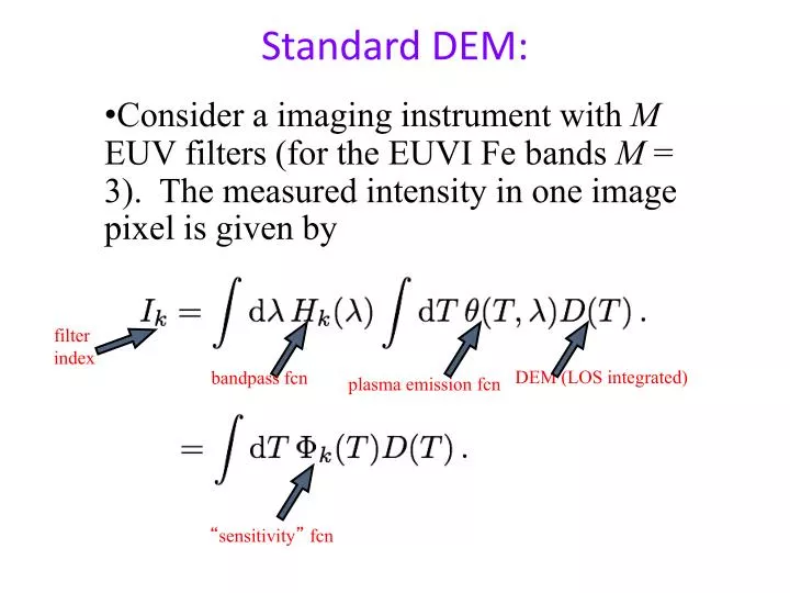
Standard DEM: • Consider a imaging instrument with M EUV filters (for the EUVI Fe bands M = 3). The measured intensity in one image pixel is given by filter index DEM (LOS integrated) bandpass fcn plasma emission fcn “sensitivity” fcn
Available data Before During After MONOCHROMATIC IMAGES: SOHO (Extreme UV) Hinode (X-ray) STEREO (Extreme UV) EIS slit direction HIGH RESOLUTION SPECTRA: Hinode/EIS (Extreme UV) Wavelength direction
Standard DEM (con’t): • The DEM D(T) is a measure of the amount of electron density (N) as a function of T along the LOS and is given by [In contrast, the new DEMT method produces a local DEM that is only integrated over a short line segment instead of the full LOS.]
Standard DEM (con’t): incl. bandpasses, atomic physics
Introduction to DEMT:What is DEMT? • Differential Emission Measure Tomography • Allows global determination of density, temperature and more in the corona (1.01 – 1.3 Rs) • Limitations: • Only a few spectral bands • time resolution of several weeks
Input: • 2-4 week time series of full-disk EUV images (EIT, EUVI, AIA, XRT) in multiple bands • Output: • 3D emissivity, local DEM N^2(r,T), irregularity factor <N^2(r)>/<N(r)>^2
DEMT, Stage 1: • Take a time series of EUV images in each of the M filters (M=3 for EUVI Fe bands). Full disk coverage will require 21 days of data when the spacecraft are separated by 90 deg. • Use tomographic processing to find the (wavelength integrated) 3D emissivity ε(r), which is related to N via:
DEMT, Stage 2: • In each pixel (centered at r), one performs a standard DEM inversion to get the temperature profile. The local DEM estimate is given by:
Results • We used STEREO A and B 171, 195 and 284 images to cover CR2069 (2008-4-16 to 5-13). Since A and B were separated by ~50 deg, we needed 23 d of data instead of 27.5. EIT was not used since it hasn’t been calibrated since 2005. • We used a 2 hr image cadence binned by 3 into 6 hour bins. This was a very comprehensive data set with no holes. • We fit a Gaussians to the tomographically determined emissivities to model the local DEM (LDEM).
Movies!!! original 1.035 1.085 1.135 synthetic
304 map1.45 Rs 195map 1.085 Rs
Region Selection (171 slice, 1.03 Rs) A C G E F B D
Newly Discovered Global Temperature Structures in the Solar Minimum Quiet Sun (submitted to ApJL) Richard Frazin, Zhenguang Huang, Enrico Landi, W.B. Manchester IV, TamasGombosi University of Michigan Alberto M. Vasquez University of Buenos Aires
First Analysis of QS loops • Quiet Sun (QS) loops have not been analyzed because they cannot be seen as distinct entities • This is not good because the QS can cover most of the Sun’s surface and due to its relatively quiescent nature should pose a more simple modeling problem than active region (AR) loops
The MLDT(Michigan Loop Diagnostic Technique) • Perform DEMT global N, T • Perform PFSSM global B • Trace the field lines through the tomographic grid, obtaining N, T at points along the field line • Repeat for thousands of field lines
Up and Down Loops After T is determined for all of the loops, we perform a fit: , where k is the voxel subscript and a,b are free If a > 0, it called a “Up” loop, and if a <0 it is called an “down” loop. Only loops with quality factor > .5 were considered
The spatial distribution of up and down loops at 1.075 $R_\odot$\ with $R^2 > .5$ for the linear temperature fit. The blue regions are threaded by down loops while the orange and dark red regions are threaded by up loops. Dark blue and dark red represent regions threaded by loops with apexes above 1.2 $\Rsun$, while light blue and orange represent loops with apexes below 1.2 $\Rsun$. The solid black line represents the boundary between open and closed field according to the PFSSM.
A 3D representation of the up and down loop geometry, with red and blue depicting up and down loops, respectively. The spherical surface has a radius at 1.035 Rsun and shows the LDEM electron temperature $T_m$\ according to the color scale.
Scale Height Analysis • The gas pressure can be determined everywhere along the loop: • The pressure scale height can then be found:
Similarly, the density scale height can be found from only the density values: • The agreement (or lack thereof) of these two scale heights is a test of the assumptions under which these laws were derived.