Fig. 3

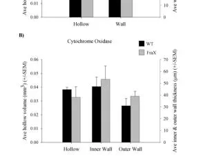
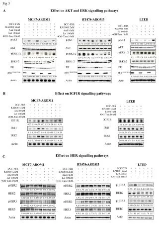
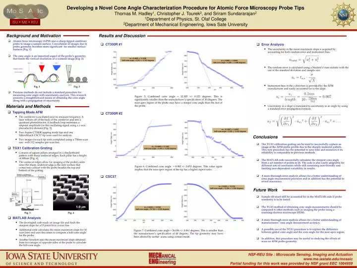
1. Developing a Novel Cone Angle Characterization Procedure for Atomic Force Microscopy Probe TipsThomas M. Hadley1, Christopher J. Tourek2, and Sriram Sundararajan21Department of Physics, St. Olaf College2Department of Mechanical Engineering, Iowa Sate University Background and Motivation Results and Discussion • Atomic force microscopy (AFM) uses a sharp-tipped cantilever probe to image a sample surface. Convolution of images due to probe geometry becomes more significant for smaller surface features [Fig. 1]. • The cone angle is an important aspect of the probe’s geometry that limits the vertical resolution of a scanned image [Fig. 2]. • Previous methods do not include a standard procedure for measuring cone angle with uncertainty analysis. This research presents a straightforward means of obtaining the cone angle along with a propagation of uncertainty. • Error Analysis • The uncertainty in the mean maximum slope is acquired by accounting for both random error and instrument bias. • The random error is calculated using a Student’s t-test statistic with the use of the standard deviation and sample size. • Instrument bias in the z direction is provided by the AFM manufacturer and easily accounted for in the slope. • Uncertainty in a slope is translated to uncertainty in an angle by using a standard error propagation formula. • CT300R #1 • CT300R #2 • CSC37 m = 9.4983 +/- 0.1638half-cone angle = 6.010 +/- 0.103 degrees m = 9.0655 +/- 0.0963half-cone angle = 6.295 +/- 0.066 degrees Fig. 1 Fig. 2 Figure 5: Combined cone angle = 12.305 +/- 0.122 degrees. This is significantly smaller than the manufacturer’s specification of 30 degrees. The near-apex region of the probe may have a steeper cone angle than the rest of the probe. Materials and Methods m = 10.3807 +/- 0.0861half-cone angle = 5.503 +/- 0.039 degrees • Tapping Mode AFM • The cantilever is oscillated near its resonant frequency. A laser reflects off of the back of the cantilever and into a quadrant photodetector. A feedback loop maintains a setpoint amplitude for this oscillating signal using a z-axis piezoelectric element [Fig. 3]. • Two Aspire CT300R tapping mode tips and one MikroMasch CSC37 tip were used for analysis. • Two images for each tip were completed using a 750nm scan size with 512 samples per scan line. • TGX1 Calibration Grating • Consists of square pillars arranged in a checkerboard pattern with sharp undercut edges. Each pillar has a height of 600nm [Fig. 4]. • The undercut edges allow for imaging of the probe’s sides since the sharp, undercut edge is the only surface that comes into contact with the probe besides the top and bottom of the grating m = 16.4486 +/- 0.1309 half-cone angle = 3.479 +/- 0.028 degrees Conclusions • The TGX1 calibration grating can be used to successfully capture an image of the AFM probe profile due to the sharply undercut pattern. This new procedure has the potential to save time and resources if its reliability is comparable to previous methods. • The MATLAB code successfully calculates the steepest cone angle from a set number of points to fit. The code is also easily adaptable for different sets of constraints while still remaining user-friendly and limiting user-dependent variability in results. • A more thorough error analysis allows for a better understanding of cone angle measurement precision and in addition has the potential to reveal inaccuracy. m = 3.6595 +/- 0.0130half-cone angle = 15.284 +/- 0.052 degrees Figure 6: Combined cone angle = 8.982 +/- 0.053 degrees. This value again implies that the near-apex region of the tip has a higher aspect ratio. m = 5.2659 +/- 0.0158 half-cone angle = 10.752 +/- 0.032 degrees Future Work • Sample tilt must still be accounted for in the MATLAB code if probe symmetry is to be tested. • The TGX1 method of obtaining cone angle measurements should be compared to other methods such as imaging the probe using a scanning electron microscope (SEM). • A more thorough error analysis allows for a better understanding of manufacturers’ cone angle measurement accuracy. • A possible use of the TGX1 procedure is to explore the difference between global cone angle and the cone angle for the near-apex region. • In addition, this procedure may be useful in studying the effects of wear on AFM probe geometry. • MATLAB Analysis • The developed code reads an image file and finds the steepest slope for a 15 point fit in a scan line. • Additional code calculates the mean maximum slope for 10 scan lines and uses this mean to compute a half-cone angle for the probe. • Another function uses the mean maximum slope obtained from two images of opposite sides of the probe to calculate the full-cone angle. Figure 7: Combined cone angle = 26.036 +/- 0.061 degrees. This is smaller than the manufacturer’s specification of 40 degrees. The tip geometry may have been altered by earlier scans using contact mode. Fig. 3 Fig. 4