Download
1 / 26
260 likes | 407 Views
Using physics when the force is complicated…. If you’re lucky, you can solve F net = m a for the new r (t) But, in general F (t) is also a function of time, and you can’t find an equation for r (t). Examples: modeling molecular dynamics Rocket propulsion

E N D
Using physics when the force is complicated… If you’re lucky, you can solve Fnet = ma for the new r(t) But, in general F(t) is also a function of time, and you can’t find an equation for r(t). Examples: modeling molecular dynamics Rocket propulsion Bacterial motion (Listeria propulsion by comet tails) Almost any real world problem! What then?
First, let’s see how you can solve a harder case of time varying force • Wind resistance and drag forces do have analytical solutions for position and velocity as a function of time! • We can also use computers to model them in general • If we use computers, then we can have arbitrarily complicated forces! • Let’s see how all this works for drag, rocketry and a real research-grade problem…
Rocket Propulsion • First, let’s talk through what forces the space shuttle experiences as a function of time: • List all the forces the shuttle experiences • Write down qualitatively how these vary as a function of time • Then, we’ll try to implement then for real…
Let’s see how a computer program can do just this, for ANY force… • Aspects of programming • Vpython • Parameters • Control structures (loops, flow control, logic) • What “=“ means in a program
Our basic approach • We know how to solve the problem when Fnet = constant. • Then x = xo + voDt + ½ a Dt2 • And so on for y and z. • How about finding x(t) for a very small time Dt • Then, during Dt, force is still (pretty much) constant • Then, compute the new force and repeat!
How to read the program: First part just sets things up and describes what I am doing: # 3D animation of rocket taking off from a flat Earth # Version 1.0 9-25-09 # Plots the trajectory of the rocket and then its distance and speed vs. time # No wind resistance in Version 1.0 from visual import * from visual.graph import * # import graphing features Any line that starts with # is just a comment The computer does nothing when it sees these—they are just to remind us what is going on! The last bits grab useful functions from a master program
Next, list what we know # initialization section # Set up the values I will need Fthrust = 32.e6 # thrust force in Newtons (average) dt = 1 # timestep in seconds m = 2.0e6 # mass in kilograms Ntimesteps = 100 # total number of timesteps for the simulation g = 9.8 # acceleration of gravity--constant at first for a flat Earth v_yo = 0. # initial speed along y axis--zero at launch v_xo = 0. # later maybe we will make it 2D! v_zo = 0. # or even 3D! x_o = 0 # initial value of x, y and z--starts at the origin y_o = 0 z_o = 0 Setup Thrust, mass, time step size Time = (# timesteps) X dt Initial values of (vo, vo , vo) at t = 0 Initial values of (xo, yo , zo) at t = 0
This part sets up our plotting and graphics rocket = cone (pos=(x_o,y_o,z_o), radius=1000, axis=(0,5000,0), color=color.white) # initialize rocket's position at (xo,yo,zo), pointing along +y rocket.velocity = vector(v_xo,v_yo,v_zo) # initialize rocket's velocity too rocket_position=[] rocket_speed=[] c = curve(pos=(x_o,y_o,z_o),color=color.red) # plots the rocket's trajectory The shuttle is plotted as a white cone Its position vector is rocket.pos It’s velocity vector is rocket.velocity A red curve indicates the shuttle’s trajectory
Now, compute the new position for each time step (while force is approximately constant) n=0 while n <= Ntimesteps: rate (20) # screen refresh rate F_net_y = Fthrust - m*g rocket_force = vector(0.,F_net_y,0.) # at first we ignore the loss of mass from fuel ejection rocket.velocity = rocket.velocity + (rocket_force/m)*dt rocket.pos = rocket.pos + rocket.velocity*dt# first update velocity, then update position second! rocket_position.append(mag(rocket.pos)) rocket_speed.append(mag(rocket.velocity)) c.append(pos=rocket.pos) n=n+1 n is called an index It counts off time steps t = n dt is the time Do what’s in the box while n < Ntimesteps First find Fnet Then use it to update velocity and position Here I just keep track of all the values I’ve computed to plot later
Finally, we plot the distance and speed vs. time # a canned functional plotting program from the vpython manual--use to plot distance and speed vs. time scene2 = display(title='Graph of position and speed') #scene2=display() # new screen with the plots funct1 = gcurve(color=color.cyan) funct2 = gcurve(delta=0.05, color=color.yellow) n=0 while n <= Ntimesteps: funct1.plot(pos=(n*dt,rocket_position[n])) # curve funct2.plot(pos=(n*dt,40.*rocket_speed[n])) # vbars n=n+1 It plots shuttle position in blue Shuttle velocity in yellow Don’t worry about how this works in detail!
OK let’s run the program!How close is our final value of rocket speed to NASA’s measured value?
Still not right…off by quite a bit.What else did we leave out?Hmmm…Can you guess?Take a minute or two to discuss and propose some ideas!
OK, include wind resistance (Version 2) New Setup information: air_density = 1.0 # air density kg/m^3 < --- correct for air pressure falling off with altitude! drag_coefficient = 0.5 # values of 0.5 to 0.75 quoted in misc. rocketry sources as the appropriate drag for this geometry (0.5 for shuttle) area = 400 # in m^2 And now the force is different: F_drag = -0.5*air_density*drag_coefficient*area*mag(rocket.velocity)*mag(rocket.velocity) F_net_y = F_thrust - m*g + F_drag
OK, now account for loss of mass as the fuel burns (Version 3.0) Yet more setup: SMME = shuttle main engine (uses liquid fuel) Solid Boosters use a different fuel source Use Dm = Dt dm/dt m = m - (dm_dt_solid+dm_dt_SMME)*dt # reduce the rocket mass by the ejected fuel
Effect of changing mass? Newton’s law is really about the law of conservation of momentum If there is no force (if a system is isolated) then: dptotal/dt = 0 Consider two objects, M and m (the rocket and its exhaust). Then: ptotal= procket + pexhaust From this we see: dptotal/dt = dprocket/dt + dpexhaust/dt = 0 Or: dprocket/dt = - dpexhaust/dt Or: Dprocket = - Dpexhaust
How to include the effect of changing mass? Now consider what happens when the rocket expels exhaust to move forward Before: ptotal= (M + m) V After: ptotal= M (V + v) + m(V–vexhaust) And before : Dprocket = - Dpexhaust M v = mvexhaust (here vexhaust is a positive speed) V M m V+v V - vexhaust M m
Main lessons: 1) Forces inside the system are equal and opposite: The rocket exerts the same force on exhaust as the exhaust exerts on the rocket (and both move in response) The Thrust (force on the rocket) is determined by the exhaust speed and the exhaust expelled per unit time: Fthrust = dpexhaust/dt = d(mvexhaust)/dt = vexhaustdm/dt 3) We need to know something more to solve for both the final rocket and exhaust speeds—you have to be given vexhaustdm/dt 4) Of course, the rocket’s mass changes as a function of time, and the thrust force can also have many different dependences on time
Finally, the thrust actually varies with time… Version 4.0 F_thrust = F_thrust_solid*(1-(F_thrust_solid-14.e6)*(n/Ntimesteps)) + (F_thrust_SMME* m_SMME/liquid_mass) # thrust varies due to the actual solid booster thrust vs. time variation: 32MN to 14 MN linear decrease over 110s, then sharp falloff to zero to end.
Still not right…off by quite a bit.What else did we leave out?Hmmm…Can you guess?Take a minute or two to discuss and propose some ideas!
Gravity changes with altitude & Air density decreases with altitude!Versions 5.0 & 6.0How big an effect are each of these?Let’s see how well it works now! air_density = exp(-mag(rocket.pos)*0.00011856) # correction for altitude Using measured data!
Listeria motion • Listeriamonocytogenesis a pathogen (disease-causing) bacterium • It moves by producing a “comet tail” of filamentous actin molecules • Experimentalists have collected movies of listeria trapped in a 2D sandwich between microscope slides and coverslips. • They move in complex ways—can we model their motion?
Actual Listeria trails (Shenoy et al. PNAS 2007)—movies @ Julie Theriot’s website • White scale bars are 5 microns long • At full speed it travels at 0.2 microns/s • Samples of its complex trails • Let’s play Newton/Kepler! • Can we find a simple model that produces all these curves from a few parameters?
Actual Listeria trails (Shenoy et al. PNAS 2007)—or see Julie Theriot’s website • Samples of its complex trails: • White scale bars are 5 microns long • At full speed it travels at 0.2 microns/s
There are competing ideas about its motion…can we really model such a complex system? Theriot lab
How to model physically? • Theriot’s group has proved that Listeria rotates as it moves along. • If a bead is attached to the bacterium’s side, the bead rotates around as the bacterium propels itself. • Let’s model its propulsion mechanism like it has a little rocket attached at one end set at a fixed angle! • This rocket rotates about the listeria’s body axis as it moves along
How would you do this? • Try to describe (maybe graphically, maybe mathematically) how you would change our program to model Listeria • Then, let’s try out a real program!