Download

1 / 59
590 likes | 679 Views
Modelling molecules using local surface properties & motion. Martyn Ford University of Portsmouth, UK martyn.ford@port.ac.uk. Atom based modelling QSAR & QSPR. Almost all modelling techniques are based on atomistic descriptions of molecules

E N D
Modelling molecules using local surface properties & motion Martyn Ford University of Portsmouth, UK martyn.ford@port.ac.uk
Atom based modellingQSAR & QSPR • Almost all modelling techniques are based on atomistic descriptions of molecules • Although these techniques have been successful over several decades, they have disadvantages • poor scaling characteristics • lack of a solid physical justification, e.g. scoring functions • interpretation difficult due to abstract nature of many descriptors • tendency to produce high dimensional models
Parasurf - a non-atom based approach • The approach is based on calculation of a set of local properties at or near the molecular surface • the local molecular electrostatic potential (MEP) • the local ionisation energy (LIE, IEL) • the local electron affinity (LEA, EAL) • the local polarisability (LP, L)
Calculation of thesurface properties • Molecules defined as isodensity surfaces • using semi-empirical AM1 electron density • can also be defined using a shrink-wrap or a marching cube algorithm • Fitted to a spherical harmonic expansion • the shape of the shrink-wrapped surface, or • the four local properties • MEP, LIE, LEA & LP
Describing surface shape:spherical harmonic expansion • The accuracy of the surface description is a function of the order L of the expansion • The greater L, the larger the computational penalty
Adjusting thesurface resolution • Spherical harmonics can be truncated at low orders for fast QSAR scans (HTS), fast superposition of molecules & rapid calculation of similarity indices • for ligands (MW < 750), L = 6-8 • for peptides & proteins (MW > 5,000), L = 25-30
Putative resolutions for in silico screening • For ligands L=6 • For receptors L=25
Advantage of this approach • The procedure gives a completely analytical description of the molecule’s shape & the 4 local properties • These 4 properties can predict the chemical and biological properties of molecules of importance in the medical, materials and environmental sciences, e.g. • intermolecular binding properties • chemical reactivity
SHCs as QSAR descriptors • The spherical harmonics coefficients (SHCs) are the parameters that define the orthogonal functions that comprise the SH expansion to any order L • For each order, there are 2L+1 coefficients • These sum to order L to give a description of the shape of a property to a required resolution
SHCs as QSAR descriptors • There are five fields (shape, MEP, LIE, LEA & LP) to be represented by five spherical harmonic expansions to order L • For high resolution (say L=15), 5 x 256 = 1280 SHCs are calculated as descriptors • This may lead to redundancy, multicollinearity & selection bias when specifying QSAR models for prediction
Selection bias • Occurs when p variables are specified from a pool of k (> p) descriptors in order to maximise the coefficient of determination (R2) or the power of prediction (Q2) • When the objective function is fit, selection bias results in upwardly biased F ratios and associated statistics (is) • as a result, the F tables used to determine significance are inappropriate (Livingstone DJ & Salt DW (2005) J.Med.Chem, 48, 661-663; Kubinyi H (Proc. EuroQSAR 2004, in press) • www.cmd.port.ac.uk/cmd/fmaxmain.shtml
How can we deal with this problem? • One approach is to use stepwise regression • We can protect against selection bias by adjusting the tail probability until random variables are prevented from entering the specified equation by chance • This can be achieved by generating 1280 uniform random variables & regressing this sample against the response variable, y
How can we deal with this problem? • The values for entering and leaving are then reduced until no random variable enters the equation • This is chosen for the model specification
Case study • Consider the following example • an aligned set of 25 D4 antagonists previously investigated using COMFA and PLS • Lanig H et al (2001) J. Med. Chem., 44, 1151 - 1157 • the study reported a 7-term QSAR equation with Q2pred = 0.74 • the range of pKi values is 4.61 to 9.21 (104.6 = 40,738 fold)
The QSAR model pKi = 3.13ar4,4 - 8.98ar9,-1 -14.75ar13,-9 - 0.79av11,-11 + 6.14 (± 0.31) (± 1.76) (± 3.27) (± 0.21) (± 0.31) where n=25, R2 = 0.90, R2adj = 0.88, Q2 = 0.82,s = 0.44,F4,20= 43.13, = 1.3 x10⁻¹⁰ This 4-term equation 1 appears to have greater power of prediction than the 7-term COMFA model reported earlier by Lanig et al (2001), for which Q2 = 0.78
Visualisation of several local properties on a single surface • Can be achieved by using RGB coding to colour code the different local properties, eg • LIE encoded on Red channel • LEA encoded on Green Channel • LP or MEP encoded on Blue Channel • This will aid interpretation & enable image analysis to be used to match compounds with similar surfaces
Allopurinol RGB Surfaces LIE encoded on Red channel LEA encoded on Green Channel LP or MEP encoded on Blue Channel
Critical points of allopurinol 8 maxima 7 minima 13 saddles No. of maxima – no. of saddles + no. of minima = Euler characteristic (S) = 2
Gradient flows & molecular surface property graphs • Characterize the behaviour of a property f : S on amolecular surface S, in terms of a directed graph G on S derived from the gradient vector field x=grad f(x) • The molecular surface property graph Gis defined by • Vertices (G) =fixed points of grad f = critical points of f • Edges (G) = stable and unstable manifolds of the saddle points
Representation of thecritical points - allopurinol • The critical points of the spherical harmonic surface descriptions can be calculated numerically • These can be visualised using RGB coding (top left) • A molecular surface graph of the van der Waals surface (top right) or some other property can be used to search databases for identity or complementarity
Amino acid surface properties • The surface properties have been calculated for the 20 naturally ocurring amino acids • using a single conformation from the Richardson Rotamer Library of experimentally observed structures
Analysing the dynamic behaviour of molecules • The approach has so far been restricted to descriptions of static molecules • How might we deal with molecular motion?
Clustering Conformations • The traditional method involves clustering conformations sampled from MD or MC simulations • However, • Linear arithmetic not appropriate for angular data • The number of clusters needs to be specified a priori • Scales as O(N2) and is therefore time consuming and restricted to small data sets!
The DASH algorithm • A time series analysis procedure • Based on circular statistics appropriate for angular data • Uses a damping function to eliminate transient, unstable states • Identifies conformers (states) using a coding system comprising strings of integers • Performs data compression for efficient storage
-180 +180 Circular Statistics Linear mean: -180 +180 Circular mean:
Elimination of unstable states • DASH has a smoothing algorithm that can remove singletons or states with a very low frequency of occurrence
Combining torsion angle state codes Coding Algorithm Individual Torsion Angle State Codes Combined Code for Conformer
Further Data Compression • The output from DASH can be further compressed to a sequence of state codes and time spent continuously in a state
Data Compression Torsion Angles from molecular dynamic simulations DASH 25000 x 8 reals 200 x 2 integers
Advantages of DASH • It can analyse torsions, distances and any calculated property • It scales linearly • wrt to the length of the simulation and number of torsion angles or distances analysed • Identifies the number of conformers and gives a unique identifier to each • Data compression • converts manyreals into a few integers • It is therefore suitable for very long simulations
Analysis of state sequences • Unlike Ward’s clustering, the sequence of states is preserved and can be used to investigate the complexity of molecular motion • illustrated for a 17 state deltamethrin MD simulation of 5 nsecs using 5 torsion angles
Modelling MD simulations • Can we model the the molecular dynamics? • Yes, using the states now identified by DASH • Why model? • To gain better understanding of the processes involved in the observed dynamic behaviour
Markov Chains • A Markov chain is a model of a stochastic process in which some variable (here the conformation code) is followed through time
Markov Chains • The probabilities of various changes between states depend only on the preceding state - 1st order Markov process • Xt = conformation code at time t Markov property
Markov Modelling • Transition probability matrix next state present state
Transition Probability Matrix Closed set
Equilibrium Distribution • At long times, MD simulations are expected to attain a unique equilibrium distribution where pi = proportion of time spent in state i.
Conformations of asparagine • Application of DASH to MD trajectories of asparagine identified six conformations with similar side chain torsion angles to the experimental structures contained in the Richardson Rotamer Library • These structures have been investigated to determine the influence of shape on surface properties