Download
1 / 149
2.65k likes | 5.56k Views
Ecological modelling. KarlineSoetaert Peter Herman Netherlands Institute of Ecology (NIOO-CEME) Yerseke, the Netherlands. Theoretical part: - course (85 pp) =>Text in boxes: not mandatory => Examples: understand how they work, make equations. Practical part: =>Modelling in EXCEL.

E N D
Ecological modelling KarlineSoetaert Peter Herman Netherlands Institute of Ecology (NIOO-CEME) Yerseke, the Netherlands • Theoretical part: - course (85 pp) • =>Text in boxes: not mandatory • => Examples: understand how they work, make equations. • Practical part: • =>Modelling in EXCEL
Ecologicalmodelling • Why modelling ? • What is a model ? • How do we make a model ? • Elementary principles • Examples
What is a model • A simplified representation of a complex phenomenon • focus only on the object of interest • ignoring the (irrelevant) details • select temporal and spatial scales of interest • Express quantitative relationships -> mathematical formulation => Predictions, tested to data • => Computers
Why do we use models • Basic research: understand in a quantitative sense how a system works; test hypotheses. • Experiments are more efficient if a model tells us what to expect • Some things cannot be directly measured (or too expensive) • If model cannot reproduce even the qualitative aspects of an observation => it is wrong => change our conceptual understanding
Why do we use models • Interpolation, budgetting: • measurements may not be accurate enough • Black-box interpolation methods do not tell us anything about the functioning of the system.
Why do we use models • Management tool: • Model predictions may be used to examine the consequences of our actions in advance. • What is the effect of REDUCING the input of organic matter to an estuary on the export of nitrogen to the sea ? • MODEL ANSWER: it INCREASES the net export. • O2 improves => denitrification lower => removal of N in estuary decreases
O2 flux (model result) C flux (sediment trap) 100 µmol cm -2 yr-1 80 Highly reactive OM (>7 /yr) 60 40 20 0 0 200 400 600 800 day cm cm cm cm cm cm cm 0 0 0 0 0 -1 0 0 5 5 5 5 5 1 1 10 10 10 10 10 2 2 NH3 15 15 NO3 15 15 O2 NO3 C 3 O2 15 C 3 20 20 20 20 4 20 4 0 20 40 0 4 8 1.2 1.8 2.4 0 80 160 0 20 40 0 1.2 1.8 2.4 80 160 % µmol liter-1 % µmol liter-1 Why do we use models • Quantification: Fitting a model to data allows quantification of processes that are difficult to measure.
Example: Westerschelde zooplankton • Question: Is there net growth of marine zooplankton species in the estuary or do they deteriorate. What is the net import/export of marine zooplankton to the estuary Fact: Difficult to measure directly (flow in/out estuary ?) Seasonal time scales, scale of km. Tool: Simplified physics, simplified biology
Ex: Westerschelde zooplankton 1. Unknown: G 2. Data: monthly transect of zooplankton biomass along a transect from the sea to the river. • Run the model assuming G=0 => Negative/positive growth • Estimate G (calibration) 3. Calculating budgets
Ex: Westerschelde zooplankton RESULT • 1. Marine zooplankton dies in the estuary; on average 5% per day; typical coastal species have lower loss rates than oceanic species • 2. Over a year, some 1500 tonnes of zooplankton dry weight is imported into the estuary each year (~4000 dutch cows).
Environmental models • Environmental models deal with the exchange of energy, mass or momentum between entities • heat transfer from the air to the water • uptake of dissolved inorganic nitrogen by phytoplankton organisms • transfer of movement from the air to the sea by the action of the wind on the sea surface
Source N Sink Elements of a model • Differential equation Time dependent:problem can be expressed by means of sources and sinks
Modelling steps • Iterative process • =>Improve if wrong • =>Data
Conceptual model • COMPONENTS: • State variable (biomass, density, concentration) • Flows or interaction • Forcing functions (light intensity, Wind, flow rates) • Ordinary variable (Grazing rates, Chlorophyll) • Parameters (ks, pFaeces) • Universal constants (e.g. atomic weights) • TEMPORAL AND SPATIAL SCALE • MODEL CURRENCY (N, C, DWT, individuals,..)
Conceptual model MODEL CURRENCY: N, -> mmol N m-3 Chlorophyll = PHYTO * [Chlorophyll/Nitrogen ratio]
Ecological interactions • deal with the exchange of energy • INTERACTION = MaximalINTERACTION * Rate limiting_Term(s) • Compartment that performs the work controls maximal strength • Rate limiting term: • a function of resource (Functional response) • a function of consumer (Carrying capacity) PREDATION (mmolC/m3/d) MaximalRate ( /d) Predator (mmolC/m3) f(Prey) (-) PREDATION = MaximalRate * Predator * f(Prey) NUTRIENTUPTAKE = MaximalRate * Algae * f(Nutrient)
Ecological interactions • Biochemical transformation: Bacteria perform work • => first-order to bacteria • => rate limiting term = function of source compartment Hydrolysis (mmolC/m3/d) MaximalHydrolysisRate ( /d) Bacteria (mmolC/m3) f(SemilabileDOC) (-) Hydrolysis = MaximalHydrolysisRate * Bacteria * f(semilabile DOC)
Ecological interactions • Rate limiting term: functional response • how a consumption rate is affected by the concentration of resource Rate=c . Resource conc Blundering idiot random encounter Low resource: ~linear High resource: handling time Low resource: ~exponential (learning,switch behavior) High resource: handling time Monod/Michaelis-Menten
Ecological interactions • More than one limiting resource: • Liebig law of the minimum: determined by substance least in supply • Multiplicative effect • preference factor for multiple food sources
Ecological interactions • CLOSURE TERMS • Models are simplicifications, not everything is explicitly modeled • => some processes are Parameterised. • Closure on mesozooplankton • => do NOT model their predators (fishes, gelatinous..) • => take into account the mortality imposed by those predators • Mesozooplankton: in mmolC/m3 • c1: /day • c2: /day/(mmolC/m3) • Mortality : mmolC/m3/day
Ecological interactions • Carrying capacity model • Rate limiting term is a function of CONSUMER • Carrying capacity is a proxy for: • Resource limitation • Predation • Space limitation
Ecological interactions • Relationships between flows • One flow = function of another flow
Inhibition • Exponential • NO3-uptake of algae inhibited by ammonium • 1-Monod • denitrification inhibited by O2
Coupled reactions INTERACTION = MaximalRate* WORK * Rate limiting_Term*Inhibition_Term
Coupled reactions • Coupling via Source-sink (previous examples) • Stoichiometry: cycles of N, C, Si, P are coupled • (CH2O)106(NH3)16(H3PO4) = C106H263O110N16P • C:H:O:N:P ratio of 106:263:110:16:1. (CH2O)106(NH3)16(H3PO4) +106 O2 ->106 CO2 +16 NH3 +H3PO4 + 106H2O • Molar ratios: • O:C ratio = 1 • N:C ratio = 16/106 • P:C ratio = 1/106
Impact of physical conditions • Currents / turbulence • pelagic constituents • benthic animals: supply of food / removal of wastes • Hydrodynamical models: coupled differential equations
Impact of physical conditions • Temperature • Rates (Physical, chemical, physiological,..) • Solubility of substances -> exchange across air-sea • Forcing function / hydrodynamical models
Impact of physical conditions • Light • Heats up water and sediment • PAR: photosynthesis • Forcing function (data/algorithm) saturation inhibition linear
Impact of physical conditions • Wind • Turbulence in water • Exchange of gasses at air-sea interface • Forcing function
Model formulation-summary • Ecological interactions: • first-order to work compartment • rate limiting terms (functional responses, carrying capacity terms) • inhibition terms • closure terms - proxy for processes not modeled • Chemical reactions • inhibition terms • Coupled models • source-sink compartments • stoichiometry • Physical conditions • currents • temperature • light • wind
NPZD model • 4 state variables - mmol N/m3 - rates per day • 1 ordinary variable: chlorophyll (calculated based on PHYTO) • 1 Forcing function: Light
NPZD model • Too simple: no temperature dependence • No sedimentation of algae / detritus
2 fundamental principles • More robust model applications • Dimensional homogeneity and consistency of units • Conservation of energy and mass
1. Consistency of units • All quantities have a unit attached • S.I. units: * m (length) * kg (mass) * s (time) * K (temperature) * mol (amount of substance) • Derived units: * C = K - 273.15 (C-1=K-1) * N = kg m s-2 (force) * J = kg m2 s-2 = N m (energy) * W = kg m2 s-3 = J s-1 (power) An equation is dimensionally homogeneous and has consistent units if the units and quantities at two sides of an equation balance
Consistency of units • To a certain extent units can be manipulated like numbers • J kg-1 = (kg m2 s-2)/kg = m2 s-2(units mass-specific energy) • Relative density of females in a population • (number of females m-2) / (total individuals m-2) = (-) • it is not allowed to add mass to length, length to area, .. • It is not allowed to add grams to kilograms • Before calculating with the numbers, the units must be written to base S.I. Units
Consistency of units • Units on both sides of the ‘=‘ sign must match => can be used to check the consistency of a model ex: the rate of change of detrital nitrogen in a water column rPHYmort = phytoplankton mortality rate (d-1) PHYC = phytoplankton concentration (mmol C m-3) NDET= detrital Nitrogen (mmol N m-3) mmol N m-3 d-1 = ( d-1) * (mmol C m-3) NOT CONSISTENT !
rPHYmort = phytoplankton mortality rate (d-1) PHYC = phytoplankton concentration (mmol C m-3) NCrPHY = Nitrogen/carbon ratio of phytoplankton (mol N (mol C)-1) Consistency of units mmol N m-3 d-1 = mmol N m-33 d-1 CONSISTENT !
2. Conservation of mass and energy • neither total mass nor energy can be created or destroyed • Sum of all rate of changes and external sources / sinks constant 3 state variables: FOOD, DAPHNIA, EGGS (mmolC/m3) 2 external sinks dDaphnia/dt+dEggs/dt+dFood/dt = Basalresp+GrowthResp+FaecesProd
2. Conservation of mass and energy If no external sources/sinks: total load must be constant. Phyto+Zoo+Fish+ Detritus+ NH3+Bottom detritus = Ct
AQUAPHY • Physiological model of unbalanced algal growth: • Algae have variable stoichiometry due to uncoupling of • photosynthesis (C-assimilation) • protein synthesis (N-assimilation) N/C (mol/mol) 0.02 0.03 0.05 0.1 0.2 0.3 Irradiance Nutrient avail
AQUAPHY • 4 state variables: Reserve, LMW, proteins (mmol C/m3), DIN (mmolN/m3)
Depth (m) 0 10 PAR 20 30 40 0 20 60 100 140 µE/m2/s Spatial components • Homogeneously mixed models: simple but not always realistic • Estuary: spread of contaminants, invasion of species: at least 1-D • Biogeochemical cycles of upper oceaneuphotic: autotrophic • Simple predator-prey models:different in spatial environment
Taxonomy of spatial models I • Landscape and patch models • Dynamics described in large number of cells Each cell: properties from GIS-> data requirements large • Real-world phenomena • Large animals • Usually statistical modellingapproach
Microscopic rules Emerging patterns Taxonomy of spatial models II • Cellular automaton models • Large number of cells • Each cell: occupied or not -> data requirements small • Interaction between neighbouring cells • Explore ecological dynamics in spatial context
Microscopic, stochastic model Macroscopic description by integration Macroscopic, continuous model Taxonomy of spatial models III • Continuous spatial models • Macroscopic approach: do not resolve individual molecules, individuals, etc.. but average over appropriate space/time and describe dynamics of the average. • Example: diffusion of molecules
Taxonomy of spatial models Probability of occurrence under this process Realisation of stochastic stationary process Express expected flux as function of concentrations (=expected occurrence prob.) Flux = - K dC/dx (Fick’s law) Count no. passing in 2 directions Difference = net flux Repeat many times Average=expected flux
unit surface M o d e InFlux l D Storage = ¶ x x Storage InFlux - OutFlux OutFlux 1-D advection-diffusion equation Consider slice with unit surface and thickness x Flux = mass passing a surface per unit time + in direction x-axis - in opposite direction