Download
1 / 46
460 likes | 630 Views
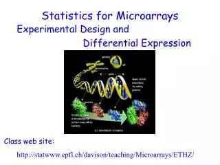
Statistics for Microarrays. Discrimination. Class web site: http://statwww.epfl.ch/davison/teaching/Microarrays/ETHZ/. Biological question Differentially expressed genes Sample class prediction etc. Experimental design. Microarray experiment. 16-bit TIFF files. Image analysis.

E N D
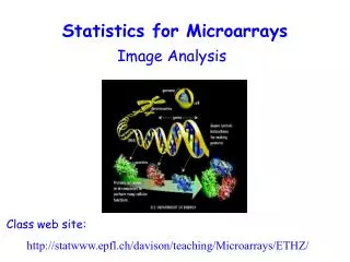
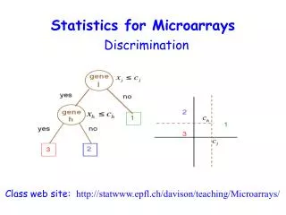
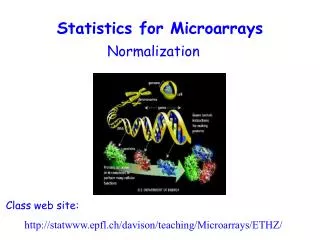
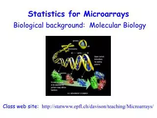
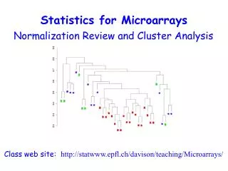
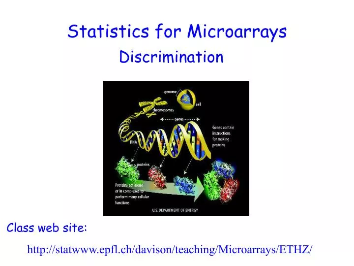
Statistics for Microarrays Discrimination Class web site: http://statwww.epfl.ch/davison/teaching/Microarrays/ETHZ/
Biological question Differentially expressed genes Sample class prediction etc. Experimental design Microarray experiment 16-bit TIFF files Image analysis (Rfg, Rbg), (Gfg, Gbg) Normalization R, G Estimation Testing Clustering Discrimination Biological verification and interpretation
cDNA gene expression data mRNA samples Data on p genes for n samples sample1 sample2 sample3 sample4 sample5 … 1 0.46 0.30 0.80 1.51 0.90 ... 2 -0.10 0.49 0.24 0.06 0.46 ... 3 0.15 0.74 0.04 0.10 0.20 ... 4 -0.45 -1.03 -0.79 -0.56 -0.32 ... 5 -0.06 1.06 1.35 1.09 -1.09 ... Genes Gene expression level of gene i in mRNA samplej = (normalized) Log(Red intensity / Green intensity)
Classification • Task: assign objects to classes (groups) on the basis of measurements made on the objects • Unsupervised: classes unknown, want to discover them from the data (cluster analysis) • Supervised: classes are predefined, want to use a (training or learning) set of labeled objects to form a classifier for classification of future observations
Discrimination • Objects (e.g. arrays) are to be classified as belonging to one of a number of predefined classes {1, 2, …, K} • Each object associated with a class label (or response) Y {1, 2, …, K} and a feature vector (vector of predictor variables) of G measurements: X = (X1, …, XG) • Aim: predict Y from X.
Example: Tumor Classification • Reliable and precise classification essential for successful cancer treatment • Current methods for classifying human malignancies rely on a variety of morphological, clinical and molecular variables • Uncertainties in diagnosis remain; likely that existing classes are heterogeneous • Characterize molecular variations among tumors by monitoring gene expression (microarray) • Hope: that microarrays will lead to more reliable tumor classification (and therefore more appropriate treatments and better outcomes)
Tumor Classification Using Gene Expression Data Three main types of statistical problems associated with tumor classification: • Identification of new/unknown tumor classes using gene expression profiles (unsupervised learning – clustering) • Classification of malignancies into known classes (supervised learning – discrimination) • Identification of “marker” genes that characterize the different tumor classes (feature or variable selection).
Classifiers • A predictor or classifier partitions the space of gene expression profiles into K disjoint subsets, A1, ..., AK, such that for a sample with expression profile X=(X1, ...,XG)Ak the predicted class is k • Classifiers are built from a learning set (LS) L = (X1, Y1), ..., (Xn,Yn) • Classifier C built from a learning set L: C( . ,L): X {1,2, ... ,K} • Predicted class for observation X: C(X,L) = k if X is in Ak
Decision Theory (I) • Can view classification as statistical decision theory: must decide which of the classes an object belongs to • Use the observed feature vector X to aid in decision making • Denote population proportion of objects of class k as pk = p(Y = k) • Assume objects in class k have feature vectors with density pk(X) = p(X|Y = k)
Decision Theory (II) • One criterion for assessing classifier quality is the misclassification rate, p(C(X)Y) • A loss function L(i,j) quantifies the loss incurred by erroneously classifying a member of class i as class j • The risk function R(C) for a classifier is the expected (average) loss: R(C) = E[L(Y,C(X))]
Decision Theory (III) • Typically L(i,i) = 0 • In many cases can assume symmetric loss with L(i,j) = 1 for i j (so that different types of errors are equivalent) • In this case, the risk is simply the misclassification probability • There are some important examples, such as in diagnosis, where the loss function is not symmetric
Maximum likelihood discriminant rule • A maximum likelihood estimator (MLE) chooses the parameter value that makes the chance of the observations the highest • For known class conditional densities pk(X), the maximum likelihood (ML)discriminant rule predicts the class of an observationX by C(X) = argmaxk pk(X)
Fisher Linear Discriminant Analysis First applied in 1935 by M. Barnard at the suggestion of R. A. Fisher (1936), Fisher linear discriminant analysis (FLDA): • finds linear combinations of the gene expression profiles X=X1,...,Xp with large ratios of between-groups to within-groups sums of squares - discriminant variables; • predicts the class of an observation X by the class whose mean vector is closest to X in terms of the discriminant variables
Gaussian ML Discriminant Rules • For multivariate Gaussian (normal) class densities X|Y= k ~ N(k,k), the ML classifier is C(X) = argmink {(X - k) k-1(X - k)’ + log| k |} • In general, this is a quadratic rule (Quadratic discriminant analysis, or QDA) • In practice, population mean vectors k and covariance matrices k are estimated by corresponding sample quantities
Gaussian ML Discriminant Rules • When all class densities have the same covariance matrix, k = the discriminant rule is linear (Linear discriminant analysis,or LDA; FLDA for k = 2): C(X) = argmink (X - k) -1(X - k)’ • When all class densities have the same diagonal covariance matrix =diag(12… G2), the discriminant rule is again linear (Diagonal linear discriminant analysis, or DLDA)
Nearest Neighbor Classification • Based on a measure of distance between observations (e.g. Euclidean distance or one minus correlation) • k-nearest neighbor rule (Fix and Hodges (1951)) classifies an observation X as follows: • find thek observations in the learning set closest to X • predict the class of X by majority vote, i.e., choose the class that is most common among those k observations. • The number of neighbors kcan be chosen by cross-validation (more on this later)
Classification Trees • Partition the feature space into a set of rectangles, then fit a simple model in each one • Binary tree structured classifiers are constructed by repeated splits of subsets (nodes) of the measurement space X into two descendant subsets (starting with X itself) • Each terminal subset is assigned a class label; the resulting partition of X corresponds to the classifier
Three Aspects of Tree Construction • Split Selection Rule • Split-stopping Rule • Class assignment Rule Different approaches to these three issues (e.g. CART: Classification And Regression Trees, Breiman et al. (1984); C4.5 and C5.0, Quinlan (1993)).
Three Rules (CART) • Splitting: At each node, choose split maximizing decrease in impurity (e.g.Gini index, entropy, misclassification error) • Split-stopping: Grow large tree, prune to obtain a sequence of subtrees, then use cross-validation to identify the subtree with lowest misclassification rate • Class assignment: For each terminal node, choose the class minimizing the resubstitution estimate of misclassification probability, given that a case falls into this node
Other Classifiers Include… • Support vector machines (SVMs) • Neural networks • Bayesian regression methods
Features • Feature selection • Automatic with trees • For DA, NN need preliminary selection • Need to account for selection when assessing performance • Missing data • Automatic imputation with trees • Otherwise, impute (or ignore)
Performance assessment (I) • Resubstitution estimation: error rate on the learning set • Problem: downward bias • Test set estimation: divide cases in learning set into two sets, L1 and L2; classifier built using L1, error rate computed for L2. L1 and L2 must be iid. • Problem: reduced effective sample size
Performance assessment (II) • V-fold cross-validation (CV) estimation: Cases in learning set randomly divided into V subsets of (nearly) equal size. Build classifiers leaving one set out; test set error rates computed on left out set and averaged. • Bias-variance tradeoff: smaller V can give larger bias but smaller variance • Out-of-bag estimation: covered below
Performance assessment (III) • Common to do feature selection using all of the data, then CV only for model building and classification • However, usually features are unknown and the intended inference includes feature selection. Then, CV estimates as above tend to be downward biased. • Features should be selected only from the learning set used to build the model (and not the entire learning set)
Aggregating classifiers • Breiman (1996, 1998) found that gains in accuracy could be obtained by aggregating predictors built from perturbed versions of the learning set; the multiple versions of the predictor are aggregated by voting. • Let C(., Lb) denote the classifier built from the bth perturbed learning set Lb, and let wbdenote the weight given to predictions made by this classifier. The predicted class for an observation x is given by argmaxk ∑b wbI(C(x,Lb) = k)
Bagging • Bagging = Bootstrap aggregating • Nonparametric Bootstrap (standard bagging): perturbed learning sets drawn at random with replacement from the learning sets; predictors built for each perturbed dataset and aggregated by plurality voting (wb = 1) • Parametric Bootstrap: perturbed learning sets are multivariate Gaussian • Convex pseudo-data (Breiman 1996)
Aggregation By-products: Out-of-bag estimation of error rate • Out-of-bag error rate estimate: unbiased • Use the left out cases from each bootstrap sample as a test set • Classify these test set cases, and compare to the class labels of the learning set to get the out-of-bag estimate of the error rate
Aggregation By-products: Case-wise information • Class probability estimates (votes) (0,1): the proportion of votes for the “winning” class; gives a measure of prediction confidence • Vote margins (–1,1) : the proportion of votes for the true class minus the maximum of the proportion of votes for each of the other classes; can be used to detect mislabeled (learning set) cases
Aggregation By-products: Variable Importance Statistics • Measure of predictive power • For each tree, randomly permute the values of the jth variable for the out-of-bag cases, use to get new classifications • Several possible importance measures
Aggregation By-products: Intrinsic Case Proximities • Proportion of trees for which cases i and j are in the same terminal node • “Clustering” • Outlier detection: 1/sum(squared proximities of cases in same class)
Boosting • Freund and Schapire (1990, 1995), Breiman (1998) • Data resampled adaptively so that the weights in the resampling are increased for those cases most often misclassified • Predictor aggregation done by weighted voting
Comparison of classifiers • Dudoit, Fridlyand, Speed (JASA, 2002) • FLDA • DLDA • DQDA • NN • CART • Bagging and boosting
Comparison study datasets • Leukemia – Golub et al. (1999) n = 72 samples, G = 3,571 genes 3 classes (B-cell ALL, T-cell ALL, AML) • Lymphoma – Alizadeh et al. (2000) n = 81 samples, G = 4,682 genes 3 classes (B-CLL, FL, DLBCL) • NCI 60 – Ross et al. (2000) N = 64 samples, p = 5,244 genes 8 classes
Leukemia data, 2 classes: Test set error rates;150 LS/TS runs
Leukemia data, 3 classes: Test set error rates;150 LS/TS runs
Lymphoma data, 3 classes: Test set error rates; N=150 LS/TS runs
Results • In the main comparison, NN and DLDA had the smallest error rates, FLDA had the highest • Aggregation improved the performance of CART classifiers, the largest gains being with boosting and bagging with convex pseudo-data • For the lymphoma and leukemia datasets, increasing the number of genes to G=200 didn't greatly affect the performance of the various classifiers; there was an improvement for the NCI 60 dataset. • More careful selection of a small number of genes (10) improved the performance of FLDA dramatically
Comparison study – Discussion (I) • “Diagonal” LDA: ignoring correlation between genes helped here • Unlike classification trees and nearest neighbors, LDA is unable to take into account gene interactions • Although nearest neighbors are simple and intuitive classifiers, their main limitation is that they give very little insight into mechanisms underlying the class distinctions
Comparison study – Discussion (II) • Classification trees are capable of handling and revealing interactions between variables • Useful by-product of aggregated classifiers: prediction votes, variable importance statistics • Variable selection: A crude criterion such as BSS/WSS may not identify the genes that discriminate between all the classes and may not reveal interactions between genes • With larger training sets, expect improvement in performance of aggregated classifiers
Additional Comparisons • Dettling and Bühlmann, improved the performance of boosting • I will let them tell you more about that!
Acknowledgements • Sandrine Dudoit • Jane Fridlyand • Yee Hwa (Jean) Yang • Terry Speed