Download
1 / 21
210 likes | 367 Views
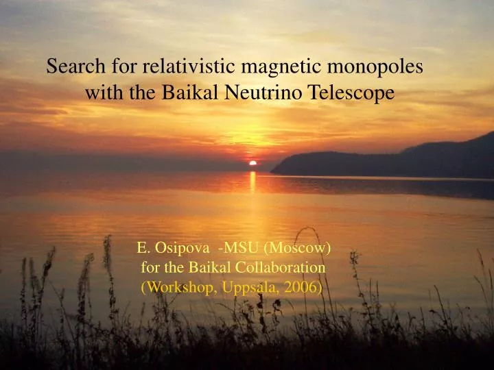
Search for relativistic magnetic monopoles with the Baikal Neutrino Telescope. E. Osipova -MSU (Moscow) for the Baikal Collaboration (Workshop, Uppsala, 2006). The Baikal Collaboration. Institute for Nuclear Research, Moscow, Russia . Irkutsk State University, Irkutsk, Russia.

E N D
Search for relativistic magnetic monopoles with the Baikal Neutrino Telescope E. Osipova -MSU (Moscow) for the Baikal Collaboration (Workshop, Uppsala, 2006)
The Baikal Collaboration Institute for Nuclear Research, Moscow, Russia. Irkutsk State University, Irkutsk, Russia. Skobeltsyn Institute of Nuclear Physics MSU, Moscow, Russia. DESY-Zeuthen, Zeuthen, Germany. Joint Institute for Nuclear Research, Dubna, Russia. Nizhny Novgorod State Technical University, Nizhny Novgorod, Russia. 7. St.Petersburg State Marine University, St.Petersburg, Russia. 8. Kurchatov Institute, Moscow, Russia.
Outline: • Introduction • Detector and Site • Search strategy for fast magnetic monopole • Atmospheric muon simulation and suppress background events • Results • Outlook
Introduction P.Dirac, 1931 g g * e = n /2 hc, n=0, ±1, ±2.. Dirac’s string If there is a monopole somewhere in the Universe, even one of such object placed anywhere would be enough to explain the quantization of electric charges B gmin =68.5 e One would be surprised if nature had made no use of it P.A.M.Dirac
Monopole mass and acceleration in magnetic fields of Universe In 1974 ‘t Hooft, Polyakov independently discovered monopole solution of the SO(3) Georgi-Glashow model Mmon ~ MV/ = 1/137 In wide classes of models Monopole mass may be in the range 107 – 1014 GeV Monopole could be accelerated up to energy 1012 –1015 GeV Monopoles with such masses may be relativistic S.Wick, T.Kephart, T.Weiler, P.Bierman Astropart.Phys. 18(2003) 663
Can monopole cross the Earth? Monopole Energy losses, crossing the Earth on diameter lg( E loss, GeV) 16 15 14 Emon= 1015 Gev E mon/M < 108 M> 107 GeV 13 12 11 10 1014GeV > Mmon > 107 GeV 0 2 4 6 8 lg (Emon/M)
Cherenkov Light from Relativistic Magnetic Monopole d Nph/dl(M) = n2 (g/e)2 d Nph/dl(muon) 8300 d Nph/dl(muon) ( n =1.33) Light flux from monopole Light flux from 10 PeV muon photons /cm β
Baikal Neutrino Telescope NT-200 192 Optical modules on 8 strings OM’s are grouped in pairs –Channel Trigger >3 Chan within 500ns OM could detect fast monopole up to 100m Expected number of hits Nhit for fast Monopole vs distance from NT200 center
Water characteristics OM response on fast monopole vs R,m Absoption Labs =22-24 m (480nm) Scattering Strongly anisotropic <cos(α)> 0.85-0.9 Lscat =30-70 m p.e. Lscat=30m Lscat=15m R,m P E from fast monopole with delay <τ for Lsc=15m, Lsc=30m OM faced to Cherenkov light (left) and in opposit side( right) Lscat 15m 30m Seff increases by 20% p.e with delay <τ p.e with delay <τ τ, ns τ, ns
Atmospheric muon simulation The main background for fast monopole signatures are muon bundles, high energy muons and shower from muons Primary particles Composition and spectral index forelements B. Wiebel-Smooth, P.Bierman, Landolt-Bornststain Cosmic Rays,6,1999, pp37-90 CORSIKA codeJ.Capdevielle et. al. KfK report (1992) QGSJET1 modelN.N Kalmykov et.al. Nucl.Phys. B52 (1997) Air shower, muons Pass at depth MUME.Bugaev et.al. Phys.Rev.D64 NT200 response to all muon energy loss processes Baikal codeI.Belolaptikovwill be published
Аtmospheric muons as standard calibration signal Time distribution t = t52-t53) MC EXP Amplitude distribution MC EXP t, ns Ph.el.
Search strategy and data analysis NT-200 1000 days of live time (April 1998-February 2002) Selection events with high multiplicity Nhit>30 To reduce the background from atmospheric muons we search for monopole from the lower hemisphere To suppress atmospheric muons a cut on time_z correlation has been applied ti ,zi - time & z-coordinates of fired channels, T,Z –their mean values per event σt ,σz - root mean square
Background suppression CUT 1 : corTZ >0 & Nhit >30 leaves 0.015% of events and reduces effective area for monopole (β=1) ~ 2 times Additional cuts after reconstruction: Cut2- Nhit>35& corTZ >0 & rec. Cut3 - Nhit>Cut2& χ2<3 Cut4 -Nhit>Cut3&θ>100o Next cuts are different for different NT200 configurations Cut5 – Cut4&Rrec>10-25 m ( Rrec -distancefrom NT200 center) Cut6- Cut5& corTZ >0.25-0.65 corTZfor atmospheric muon (black-EXP, red-MC) and for fast monopole from the lower hemisphere (blue) No events from experimental sample pass CUTS 1-6
The main sources of background CUT1 CUT3 CUT4 CUT5 Simulated atmospheric muons satisfying CUT1 vs cascade energy(upper) and vs number of muons in bundle(lower) The events with a large number of muons in bandle are supressed after reconstruction with χ2<3 MC events lg(Esh,TeV) Number of muons in bundle Number of muons in bundle Lg(Esh,TeV
Comparison of experimental and MC data with respect toparameters which used for background rejection for events satisfying CUT1 Distance from NT200 center Reconstructed θ MC EXP Expected from monopole R, m θ, grad Simulation describes EXP data quite well even for very rare events. Number of fired channels
Passing rates versus Cut-level MC EXP Seff for monopole (β=1) Passing rates Effective area for fast monopole (β=1) decrease 2 times from CUT1 –CUT6 CUT level
90% C.L. upper limit on the flux of fast monopole (1000livedays NT200) Upper limit on the flux of fast monopole From the non-observation of candidate events in NT200 an upper limit on the flux of fast monopole is obtained Acceptance & Upper flux limit
Outlook NT200+=NT200 +3 external string ( 36OMs) NT200+ put into operation in 2005. The main advantage of NT200+ is the possibility to select cascades. It allows to reject background using more soft cuts. We expect increasing effective area for fast monopole at 1.5 times comparing NT200 • - Height = 210m • = 200m • Volume ~ 4 Mton
A future Gigaton Volume Detector (Baikal-GVD) Sparse instrumentation: 90 – 100 strings 300 – 350 m lengths with 12 - 16 OM per string = 1300 - 1700 OMs (NT200 = 192 OMs) distance between strings 100 m Expected sensitivity for fast monopole (1 year GVD) Fmon< 5 · 10-18 cm-2 s-1 sr-1 Top view of the planned Baikal-GVD detector. Also shown is basic cell: a “minimized” NT200+ telescope
CONCLUSION • BAIKAL Experimenal Upper limit on the Fast ( v/c =1) Monopole Flux • (90% C.L) • Fmon < 0.46 ·10-16 cm-2sec-1 sr-1 • The limit on fast magnetic monopole flux obtained in this analysis is the best • at the present time • 2. NEW configuration NT200+ • Permits to reject background using more soft cuts. Expected 1.5 times increase • of effective area for fast monopole comparing NT200 • 3. Gigaton Volume (km3-scale) Detector (Baikal-GVD) • Expected sensitivity for fast monopole (1 year operation) • Fmon< 5 · 10-18 cm-2 s-1 sr-1
Baikal Baikal Water characteristics Absorption and Scattering cross-section vs λ Absoption Scattering Strongly anisotropic <cos(α)> 0.85-0.9 Lscat=30-70 m Labs =22-24 m Lscat 15m 30m Seff increases by 20% OM responce vs R,m OM faced opposit Cherenkov light OM faced to Cherenkov light p.e. p.e. p.e with delay <τ p.e with delay <τ R,m τ, ns τ, ns