Download
1 / 49
510 likes | 514 Views
Processors and Memory Hierarchy. Architectural Distinctions. Architectural distinctions between modern CISC and traditional RISC processors are shown in Figure 4.4 The main features of the RISC and CISC processors are compared in Table 4.2. There are five areas for comparison: Instruction sets

E N D
Architectural Distinctions • Architectural distinctions between modern CISC and traditional RISC processors are shown in Figure 4.4 • The main features of the RISC and CISC processors are compared in Table 4.2. There are five areas for comparison: • Instruction sets • Addressing modes • Register file and cache design • Clock rate and expected CPI • Control mechanism
CISC Scalar Processors • A scalar processor executes with scalar data. The simplest scalar processor executes integer instructions using fixed-point operands. More capable scalar processors execute both integer and floating-point operations. A modern scalar processor may possess both an integer unit and a floating-point unit in the same CPU.
Representative CISC Processors • In Table 4.3, three representative CISC scalar processors are listed. The VAX 8600 processor is built on a PC board. The i486 and M68040 are single-chip microprocessors. They are still widely used at present. We use these popular architectures to explain some interesting features built into modern-CISC machines.
RISC Scalar Processors • Generic RISC processors are called scalar RISC because they are designed to issue one instruction per cycle, similar to the base scalar processor shown in Fig. 4.2a. In theory, both RISC and CISC scalar processors should perform about the same if they run with the same clock rate and with equal program length. However, these two assumptions are not always valid, as the architecture affects the quality and density of code generated by compilers. • The RISC design gains its power by pushing some of the less frequently used operations into software.
Representative RISC Processors • Four RISC-based processors, the Sun SPAPC, Intel i860, Motorola M88100, and AMD 29000, are summarized in Table 4.4. All of these processors use 32-bit instructions. The instruction sets consist of 51 to 124 basic instructions. On-chip floating-point units are built into the, i860 and M88100, while.the SPARC and AMD use off-chip floating-point units. We consider these four processors generic scalar RISC issuing essentially only one instruction per pipeline cycle.
Superscalar and Vector Processors • A CISC or a RISC scalar processor can be improved with a superscalar or vector architecture. Scalar processors are those executing one instruction per cycle. • In a superscalar processor, multiple instruction pipelines are used. This implies that multiple instructions are issued per cycle and multiple results are generated per cycle.
Superscalar Processors • Superscalar processors are designed to exploit more instruction-level parallelism in user programs. Only independent instructions can be executed in parallel without causing a wait state. The amount of instruction-level parallelism varies widely depending on the type of code being executed.
Pipelining in Superscalar Processors • The fundamental structure of a superscalar pipeline is illustrated in Fig. 4.11. • In order to fully utilise a superscalar processor of degree m, m instructions must be executable in parallel. This situation may not be true in all clock cycles. In that case, some of the pipelines may be stalling in a wait state. • In a superscalar processor, the simple operation latency should require only one cycle, as in the base scalar processor.
The VLIW Architecture • The VLIW architecture is generalized from two well-established concepts: horizontal microcoding, and superscalar processing. A typical VLIW (very long instruction word) machine has instruction words hundreds of bits in length. As illustrated in Fig. 4.14a, multiple functional units are used concurrently in a VLIW processor. All functional units share the use of a common large register file. The operations to be simultaneously executed by the functional units are synchronized in a VLIW instruction, say, 256 or 1024 bits per instruction word, as implemented in the Multiflow computer models.
Pipelining in VLIW Processors • The execution of instructions by an ideal VLIW processor was shown in Fig. 4.14b. VLIW machines behave much like superscalar machines with three differences: • First, the decoding of VLIW instructions is easier than that of superscalar instructions. • Second, the code density of the superscalar machine is better when the available instruction-level parallelism is less than that exploitable by the VLIW machine. • Third, a superscalar machine can be object-code-compatible with a large family nonparallel machines. On the contrary, a VLIW machine exploiting different amounts of parallelism would require different instruction sets.
Memory Hierarchy Technology • Storage devices such as registers, caches, main memory, disk devices, and tape units are often organised as a hierarchy as depicted in Fig. 4.17. The memory technology and storage organisation at each level are characterised by five parameters: • access time (ti) • memory size (si) • cost per byte (ci) • transfer bandwidth (bi) • unit of transfer (xi).
Memory Hierarchy Technology (cont.) • The access time ti refers to the round-trip time from the CPU to the ith-level memory. • The memory size si is the number of bytes or words in level i. • The cost of the ith-level memory is estimated by the product cisi. • The bandwidth bi refers to the rate at which information is transferred between adjacent levels. • The unit of transfer xi refers to the grain size for data transfer between levels i and i + 1.
Peripheral Technology • Besides disk drives and tape units, peripheral devices include printers, plotters, terminals, monitors, graphics displays, optical scanners, image digitizers, output microfilm devices, etc. Some I/O devices are tied to special-purpose or multimedia applications.
Hierarchical memory structure • The objective of hierarchical memory in PPAs & multiprogrammed uniprocessor systems are: • match processor speed memory B/W • Reduce the potential conflicts at each level of the hierarchy
Memory Classification • Classification of memories according to several attributes: • Accessing method: • RAM (Random Access Memory) • SAM (Sequential Access Memory) • DASD (Direct Access Storage Devices) • Access time • Primary memory (RAMs) • Secondary memory (DASDs & optimal SAMs)
Optimization of Memory Hierarchy • The goal in designing an n-level memory hierarchy is to achieve a: • Performance close to that of the fastest memory • Cost per bit close to that of the cheapest memory • Performance depends on: • Program behaviour with respect to memory References • Access time & memory size of each level • Granularity of info transfer (block size) • Management policies • Design of processor-memory interconnected network
Optimization of Memory Hierarchy (cont. • A typical memory hierarchy design problem involves an optimisation which minimises the effective hierarchy access time T, subject to a given memory system cost Co & size constraints. • That is, minimize: • Subject to the constraints
Inclusion, Coherence, and Locality • Information stored in a memory hierarchy (M1, M2, ... , Mn) satisfies three important properties: inclusion, coherence, and locality as illustrated in Fig. 4.18. We consider cache memory the innermost level M1, which directly communicates with the CPU registers. The outermost level Mn contains all the information words stored.
Inclusion Property • The inclusion property is stated as • The set inclusion relationship implies that all information items are originally stored in the outermost level Mn. During the processing, subsets of Mn are copied into Mn-1. Similarly, subsets of Mn-1, are copied into Mn-2, and so on.
Coherence Property • The coherence property requires that copies of the same information item at successive memory levels be consistent. If a word is modified in the cache, copies of that word must be updated immediately or eventually at all higher levels. The hierarchy should be maintained as such. • The first method is called write-through (WT), which demands immediate update in Mi+l if a word is modified in for i = 1, 2, ... , n – 1. • The second method is write-back (WB), which delays the update in Mi+1 until the word being modified in Mi is replaced or removed from Mi.
Locality of References • The memory hierarchy was developed based on a program behaviour known as locality of references. Memory references are generated by the CPU for either instruction or data access. • There are three dimensions of the locality property: • Temporal locality • Spatial locality • Sequential locality
Memory Capacity Planning • The performance of a memory hierarchy is determined by the effective access time Teff to any level in the hierarchy. • It depends on the hit ratios and access frequencies at successive levels.
Hit Ratios • The hit ratios at successive levels are a function of: • memory capacities • management policies • program behavior • The access frequency to Mi is defined as fi = (1-h1)(1 - h2)...(1 - hi-1)hi. This is indeed the probability of successfully accessing Mi when there are i - 1 misses lower levels and a hit at Mi. Note that and fl = h1.
Effective Access Time • Using the access frequencies fi for i = 1, 2,..., n, we can formally define the effective access time of a memory hierarchy as follows: • Teff = = h1t1 + (1-h1)h2t2 +...+(1-h1)(1-h2)...(1-hn-1)tn
Hierarchy Optimization • The total cost of a memory hierarchy is estimated as follows:
Hierarchy Optimization (cont.) • The optimisation process can be formulated as a linear programming problem, given a ceiling C0 on the total cost - that is, a problem to minimise (4.5) • subject to the following constraints:si > 0, ti > 0 for i = 1,2, ... n
Addressing Schemes for main memory • Main memory is partitioned into several independent memory modules and the addresses distributed across these modules. • This scheme, called interleaving, resolves some of the interference by allowing concurrent accesses to more than one module. • There are 2 basic methods of distributing the addresses among the memory modules: • high-order interleaving Fig. 2.3 • Low-order interleaving Fig. 2.4
Virtual Memory System • In many applications, large programs cannot fit in main memory for execution. • The natural solution is to introduce management schemes that intelligently allocate portions of memory to users as necessary for the efficient running of their programs.
Virtual Memory Models • The idea is to expand the use of the physical memory among many programs with the help of an auxiliary (backup) memory such as disk arrays. • Only active programs or portions of them become residents of the physical memory at one time. The vast majority of programs or inactive programs are stored on disk.
Address Spaces • Each word in the physical memory is identified by a unique physical address. All memory words in the main memory form a physical address space. Virtual addresses are generated by the processor during compile time. • The virtual addresses must be translated into physical addresses at run time. A system of translation tables and mapping functions are used in this process.
Address Mapping • Let V be the set of virtual addresses generated by a program (or by a software process) running on a processor. • Let M be the set of physical addresses allocated to run this program. • A virtual memory system demands an automatic mechanism to implement the following mapping:
Private Virtual Memory • Each private virtual space is divided into pages. • Virtual pages from different virtual spaces are mapped into the same physical memory shared by all processors.
Shared Virtual Memory • This model combines all the virtual address spaces into a single globally shared virtual space (Fig. 4.20b). • Each processor is given a portion of the shared virtual memory to declare their addresses. • Different processors may use disjoint spaces. • Some areas of virtual space can be also shared by multiple processors.
Address Translation Mechanisms • The process demands the translation of virtual addresses into physical addresses. • Various schemes for virtual address translation are summarised in Fig. 4.21a. • The translation demands the use of translation maps which can be implemented in various ways.
Translation Lookaside Buffer • Translation maps appear in the form of a translation lookaside buffer (TLB) and page tables (PTs). • The TLB is a high-speed lookup table that stores the most recently referenced or likely referenced page entries. • The use of a TLB and PTs for address translation is shown in Fig 4.21b. Each virtual address is divided into three fields: • The leftmost virtual page number • The middle cache block number • The rightmost word address
Paged Segments • The two concepts of paging and segmentation can be combined to implement a type of virtual memory with paged segments. • Within each segment, the addresses are divided into fixed-size pages.
Inverted Paging • The direct paging described above works well with a small virtual address space such as 32 bits. In modern computers, the virtual address space is very large, such as 52 bits in the IBM RS/6000. • Besides direct mapping, address translation maps can also be implemented with inverted mapping (Fig. 4.21c). • The generation of a long virtual address from a short physical address is done with the help of segment registers, as demonstrated in Fig. 4.21c.
Example 4.8: • As with its predecessor in the 80x86 family, the i486 features both segmentation and paging compatibilities. • A segment can start at any base address, and storage overlapping between segments is allowed. The virtual address (Fig. 4.22a) has a 16-bit segment selector to determine the base address of the linear address space to be used with the i486 paging system. • The paging feature is optional on the i486. • A 32-entry TLB (Fig 4.22b) is used to convert the linear address directly into the physical address without resorting to the two-level paging scheme (Fig 4.22c).
Memory Management • The various memory management techniques include: • Fixed-partition • Dynamic • Virtual -> segmentation & paging • Memory management is concerned with the following functions: • Keeping track of the status of each location • Determining the allocation policy for memory • Allocation : status info must be updated • Deallocation: release of previously allocated memory
Program relocation • During the execution of a program, the processor generates logical addresses which are mapped into the physical address space in main memory. • The address mapping is performed: • when the program is initially loaded (static relocation) • During the execution of the program (dynamic relocation)
Disadvantages of static relocation • Makes it difficult for processors to share info which is modifiable during execution • If a program is displaced from main memory by mapping, it must be reloaded into the same set of memory locations -> binding the physical address space of the program for the duration of the execution -> inefficient
Address map implementation • Direct mapping: not efficient -> slow • Associative mapping: uses associative memory (AM) that maintains the mapping between recently used virtual and physical memory addresses.
Three methods of mapping VM ->MM • Paged memory system: virtual space is partitioned into pages with matching size blocks in memory. • Virtual address: • virtual page # • displacement • Segmented memory system: programs which are block-structured & written in Pascal, C, & Algol yield a high degree of modularity. • Paged segments
Memory Replacement Policies • Memory management policies include the allocation and deallocation of memory pages to active processes and the replacement of memory pages. • Page replacement refers to the process in which a resident page in main memory is replaced by a new page transferred from the disk.
Page Traces • To analyse the performance of a paging memory system, page trace experiments are often performed. • A page trace is a sequence of page frame numbers (PFNs) generated during the execution of a given program. Each PFN corresponds to the prefix portion of a physical memory address. By tracing the successive PFNs in a page trace against the resident page numbers in the page frames, one can determine the occurrence of page hits or of page faults. • A page trace experiment can be performed to determine the hit ratio of the paging memory system.
Page Replacement Policies • The following page replacement policies are specified in a demand paging memory system for a page fault at time t. • Least recently used (LRU) • Optimal (OPT) algorithm • First-in-first-out (FIFO) • Least frequently used (LFU) • Circular FIFO • Random replacement
Examples of memory management allocation policies • Least Recently Used (LRU)- replaces the page with the largest backward distance <popular> • Belady's Optimal Algorithm (MIN)- replaces the page with the largest forward distance • Least Frequently Used (LFU)- replaces the page that has been referenced the least # of times. • First-In, First-Out (FIFO)- replaces the page that has been in memory for the longest time. • Last-In, First-Out (LIFO)- replaces the page that has been in memory for the shortest time. • Random (RAND)- chooses a page at random for replacement