Download
1 / 45
480 likes | 765 Views
Memory Hierarchy. Ali Azarpeyvand Advanced Computer Architecture. Review: Summary. Instruction Level Parallelism (ILP) in SW or HW Loop level parallelism is easiest to see SW parallelism dependencies defined for program, hazards if HW cannot resolve

E N D
Memory Hierarchy Ali Azarpeyvand Advanced Computer Architecture
Review: Summary • Instruction Level Parallelism (ILP) in SW or HW • Loop level parallelism is easiest to see • SW parallelism dependencies defined for program, hazards if HW cannot resolve • SW dependencies/compiler sophistication determine if compiler can unroll loops • Memory dependencies hardest to determine • HW exploiting ILP • Works when can’t know dependence at run time • Code for one machine runs well on another • Key idea of Scoreboard: Allow instructions behind stall to proceed (Decode => Issue instr & read operands) • Enables out-of-order execution => out-of-order completion • ID stage checked both for structural and WAW
Review: Summary • Branch Prediction • Branch History Table: 2 bits for loop accuracy • Recently executed branches correlated with next branch? • Branch Target Buffer: include branch address & prediction • Predicated Execution can reduce number of branches, number of mispredicted branches • Speculation: Out-of-order execution, In-order commit (reorder buffer) • SW Pipelining • Symbolic Loop Unrolling to get most from pipeline with little code expansion, little overhead • Superscalar and VLIW: CPI < 1 (IPC > 1) • Dynamic issue vs. Static issue • More instructions issue at same time => larger hazard penalty
Outline • Memory hierarchy • Principle of locality • Cache types • Questions: • Q1: Where can a block be placed in the upper level? (Block placement) • Q2: How is a block found if it is in the upper level? (Block identification) • Q3: Which block should be replaced on a miss? (Block replacement) • Q4: What happens on a write? (Write strategy)
Control Datapath The Big Picture: Where are We Now? • The Five Classic Components of a Computer • This lecture (and next few): Memory System Processor Input Memory Output
µProc 60%/yr. (2X/1.5yr) 1000 CPU “Moore’s Law” 100 Processor-Memory Performance Gap:(grows 50% / year) Performance 10 DRAM 9%/yr. (2X/10 yrs) DRAM 1 1980 1981 1982 1983 1984 1985 1986 1987 1988 1989 1990 1991 1992 1993 1994 1995 1996 1997 1998 1999 2000 Time Recap: Who Cares About the Memory Hierarchy? Processor-DRAM Memory Gap (latency)
Memory System Processor DRAM Cache The Motivation for Caches • Motivation • Large (cheap) memories (DRAM) are slow • Small (costly) memories (SRAM) are fast • Make the average access time small • service most accesses from a small, fast memory • reduce the bandwidth required of the large memory
Frequency of reference 0 Address Space 2n The Principle of Locality • The Principle of Locality • Program accesses a relatively small portion of the address space at any instant of time • Example: 90% of time in 10% of the code • Two different types of locality • Temporal Locality (locality in time): • if an item is referenced, it will tend to be referenced again soon • Spatial Locality (locality in space): • if an item is referenced, items close by tend to be referenced soon
Generations of Microprocessors • Time of a full cache miss in instructions executed: 1st Alpha: 340 ns/5.0 ns = 68 clks x 2 or 136 2nd Alpha: 266 ns/3.3 ns = 80 clks x 4 or 320 3rd Alpha: 180 ns/1.7 ns =108 clks x 6 or 648
Area Costs of Caches Processor % Area %Transistors (cost) (power) • Intel 80386 0% 0% • Alpha 21164 37% 77% • StrongArm SA110 61% 94% • Pentium Pro 64% 88% • 2 dies per package: Proc/I$/D$ + L2$ • Itanium 92% • Caches store redundant dataonly to close performance gap
Levels of the Memory Hierarchy Upper Level Capacity Access Time Cost Staging Xfer Unit faster CPU Registers 100s Bytes <10s ns Registers prog./compiler 1-8 bytes Instr. Operands Cache K Bytes 10-100 ns 1-0.1 cents/bit Cache cache cntl 8-128 bytes Blocks Main Memory M Bytes 200ns- 500ns $.0001-.00001 cents /bit Memory OS 512-4K bytes Pages Disk G Bytes, 10 ms (10,000,000 ns) 10 - 10 cents/bit Disk -6 -5 user/operator Mbytes Files Larger Tape infinite sec-min 10 Tape Lower Level -8
Many Levels in Memory Hierarchy Invisible only to high-levellanguage programmers Pipeline registers Register file There can also bea 3rd (or more) cache levels here 1st-level cache(on-chip) Usually madeinvisible tothe programmer(even assemblyprogrammers) 2nd-level cache(on same MCM as CPU) Our focusin this lecture Physical memory(usu. mounted on same board as CPU) Virtual memory(on hard disk, often in same enclosure as CPU) Disk files(on hard disk often in same enclosure as CPU) Network-accessible disk files(often in the same building as the CPU) Tape backup/archive system(often in the same building as the CPU) Data warehouse: Robotically-accessed room full of shelves of tapes (usually on the same planet as the CPU)
Simple Hierarchy Example • Note many orders of magnitude change in characteristics between levels:
The Principle of Locality • The Principle of Locality: • Program access a relatively small portion of the address space at any instant of time. • Two Different Types of Locality: • Temporal Locality (Locality in Time): If an item is referenced, it will tend to be referenced again soon (e.g., loops, reuse). • Spatial Locality (Locality in Space): If an item is referenced, items whose addresses are close by tend to be referenced soon(e.g., straightline code, array access).
Lower Level Memory Upper Level Memory To Processor Blk X From Processor Blk Y Memory Hierarchy: Terminology • Hit: data appears in some block in the upper level (example: Block X) • Hit Rate: the fraction of memory access found in the upper level • Hit Time: Time to access the upper level which consists of RAM access time + Time to determine hit/miss • Miss: data needs to be retrieved from a block in the lower level (Block Y) • Miss Rate = 1 - (Hit Rate) • Miss Penalty: Time to replace a block in the upper level + Time to deliver the block the processor • Hit Time << Miss Penalty • Block: A fixed-size collection of data containing the requested word
Cache Measures • Hit rate: fraction found in that level • So high that usually talk about Miss rate • Average memory-access time = Hit time + Miss rate x Miss penalty (ns or clocks) • Miss penalty: time to replace a block from lower level, including time to transfer to CPU • access time: time to lower level = f(latency to lower level) • transfer time: time to transfer block =f(BW between upper & lower levels)
4 Questions for Memory Hierarchy • Q1: Where can a block be placed in the upper level? (Block placement) • Q2: How is a block found if it is in the upper level? (Block identification) • Q3: Which block should be replaced on a miss? (Block replacement) • Q4: What happens on a write? (Write strategy)
4 Byte Direct Mapped Cache Cache Index 0 1 2 3 Simplest Cache: Direct Mapped Memory Address Memory 0 • Location 0 can be occupied by data from: • Memory location 0, 4, 8, ... etc. • In general: any memory locationwhose 2 LSBs of the address are 0s. • Address<1:0> => cache index. • Which one should we place in the cache? • How can we tell which one is in the cache? 1 2 3 4 5 6 7 8 9 A B C D E F
31 10 4 0 Cache Tag Example: 0x50 Cache Index Byte Select Ex: 0x01 Ex: 0x00 Stored as part of the cache “state” Valid Bit Cache Tag Cache Data : Byte 31 Byte 1 Byte 0 0 : 0x50 Byte 63 Byte 33 Byte 32 1 2 3 : : : : Byte 2047 Byte 2016 63 2 KB Direct Mapped Cache, 32B blocks • For a 2 ** N byte cache, 32-bit address: • The uppermost (32 - N) bits are always the Cache Tag • The lowest M bits are the Byte Select (Block Size = 2 ** M) • Our example: Address: 0x28020 = 000000000000001010000 00000100000 N=11, M=5, N-M=6
Advantage. Simple hardware decision for replacement Low cost. It doesn't need replacement algorithm. Disadvantage: See example. Direct Mapped Cache Address: 16 bit, 16-Byte blocks
Example Repeat. Call get data ; compiled in block x of memory. Call compare ; compiled in block x+128 of memory. Until match or end_of_data. ___________________________________________. Both blocks must be mapped to block x of cache, so miss will occur whenever the repeat-until loop executes.
FULLY_ASSOCIATIVE. Advantages: NO limitation in block mapping. Possibility of using different replacement algorithms. NO relation between the number of memory blocks and cache blocks. Disadvantage: Higher cost, because of the need to search of all tags. Fully Associative
Combination of direct and associative mapping techniques. The contention problem of directmethod is eased. The hardware cost is reduced by decreasing the size of associative search. Set Associative
Cache Index Valid Cache Tag Cache Data Cache Data Cache Tag Valid Cache Block 0 Cache Block 0 : : : : : : Adr Tag Compare Compare 1 0 Mux Sel1 Sel0 OR Cache Block Hit Two-way Set Associative Cache • N-way set associative: N entries for each Cache Index • N direct mapped caches operates in parallel (N typically 2 to 4) • Example: Two-way set associative cache • Cache Index selects a “set” from the cache • The two tags in the set are compared in parallel • Data is selected based on the tag result
Cache Index Valid Cache Tag Cache Data Cache Data Cache Tag Valid Cache Block 0 Cache Block 0 : : : : : : Adr Tag Compare Compare 1 0 Mux Sel1 Sel0 OR Cache Block Hit Disadvantage of Set Associative Cache • N-way Set Associative Cache v. Direct Mapped Cache: • N comparators vs. 1. • Extra MUX delay for the data. • Data comes AFTER Hit/Miss. • In a direct mapped cache, Cache Block is available BEFORE Hit/Miss: • Possible to assume a hit and continue. Recover later if miss.
Cache Size Equation • Simple equation for the size of a cache: • (Cache size) = (Block size) × (Number of sets) × (Set Associativity) • Can relate to the size of various address fields: • (Block size) = 2(# of offset bits) • (Number of sets) = 2(# of index bits) • (# of tag bits) = (# of memory address bits) (# of index bits) (# of offset bits) Memory address
Q1: Where can a block be placed in the upper level? • Block 12 placed in 8 block cache: • Fully associative, direct mapped, 2-way set associative • S.A. Mapping = Block Number Modulo Number Sets (n-way set associative)
Q2: How is a block found if it is in the upper level? • Tag on each block • No need to check index or block offset • Increasing associativity • shrinks index • expands tag
Q3: Which block should be replaced on a miss? • Easy for Direct Mapped • Set Associative or Fully Associative: • Random • LRU (Least Recently Used) • Block that has been unused for the longest time. • FIFO (First In First Out) • LFU (Least Frequently used) Data cache misses per 1000 instructions
Writes Vs. Reads • Reads are more common. • data access: • 10% stores and 37% loads for MIPS programs, • making writes 10%/(100% + 37% + 10%) or about 7% of the overall memory traffic. • Or 10%/(37%+10%) or 21% of data cache traffic. • Make the common case fast: Read. • The block can be read the same time the tag is read and compared. (for DM) • Embedded processors might not like this. • This optimization is not valid for write. • Where to write the data if the block is found in cache?
What Happens on Writes • Write through: new data is written to both the cache block and the lower-level memory. • Help to maintain cache consistency. • Write back: new data is written only to the cache block. • Lower-level memory is updated when the block is replaced. • A dirty bit is used to indicate the necessity. • Help to reduce memory traffic. • What happens if the block is not found in cache?
Write Allocation • Write allocate: Fetch the block into cache, then write the data (usually combined with write back). • No-write allocate: Do not fetch the block into cache (usually combined with write through). • Pros and Cons of each? • WT: read misses cannot result in writes. • WB: no repeated writes to same location. • WT always combined with write buffers so that don’t wait for lower level memory.
Write Buffer for Write Through Cache Processor DRAM • A Write Buffer is needed between the Cache and Memory • Processor: writes data into the cache and the write buffer • Memory controller: write contents of the buffer to memory • Write buffer is just a FIFO: • Typical number of entries: 4 • Works fine if: Store frequency << 1 / DRAM write cycle • Memory system designer’s nightmare: • Store frequency -> 1 / DRAM write cycle • Write buffer saturation Write Buffer
Basics of Cache Operation Through Back
Real Example: Alpha 21264 Caches • 64KB 2-way associative instruction cache • 64KB 2-way associative data cache I-cache D-cache
Instruction vs. Data Caches • Instructions and data have different patterns of temporal and spatial locality • Also instructions are generally read-only • Can have separate instruction & data caches • Advantages • Doubles bandwidth between CPU & memory hierarchy • Each cache can be optimized for its pattern of locality • Disadvantages • Slightly more complex design • Can’t dynamically adjust cache space taken up by instructions vs. data
Cache Performance Equations • Memory stalls per program (blocking cache): • CPU time formula: • More cache performance will be given later!
Cache Performance Example • Ideal CPI=2.0, memory references / inst=1.5, cache size=64KB, miss penalty=75ns, hit time=1 clock cycle • Compare performance of two caches: • Direct-mapped (1-way): cycle time=1ns, miss rate=1.4% • 2-way: cycle time=1.25ns, miss rate=1.0%
Out-Of-Order Processor • Define new “miss penalty” considering overlap • Compute memory latency and overlapped latency • Example (from previous slide) • Assume 30% of 75ns penalty can be overlapped, but with longer (1.25ns) cycle on 1-way design due to Out-of-Order
Cache Measures • Hit rate: fraction found in that level • So high that usually talk about Miss rate • Average memory-access time = Hit time + Miss rate x Miss penalty (ns or clocks) • Miss penalty: time to replace a block from lower level, including time to transfer to CPU • access time: time to lower level = f(latency to lower level) • transfer time: time to transfer block =f(BW between upper & lower levels)
Cache Performance • Average memory access time = Hit time + miss rate * miss penalty • Memory stall cycles: the number of cycles during which the CPU is stalled waiting for a memory access • CPU time =( CPU execution clock cycles + Memory stall cycles) * clock cycle time • Memory stall clock cycles = Number of misses x Miss penalty = Reads * read miss rate * read miss penalty + Writes * write miss rate * write miss penalty
Cache Performance Improvement (Average memory access time) = (Hit time) + (Miss rate)×(Miss penalty) • Reduce miss penalty: • Multilevel cache; Critical word first and early restart; priority to read miss; Merging write buffer; Victim cache • Reduce miss rate: • Larger block size; Increase cache size; Higher associativity; Way prediction and Pseudo-associative caches; Compiler optimizations • Reduce miss penalty/rate via parallelism: • Non-blocking cache; Hardware and Compiler-controlled prefetching • Reduce hit time: • Small simple cache; Avoid address translation in indexing cache; Pipelined cache access; Trace caches