Download
1 / 23
270 likes | 1.12k Views
Band Pass Systems, Phasors and Complex Representation of Systems. KEY LEARNING OBJECTIVES. I. Phasors (complex envelope) representation for sinusoidal signal narrow band signal. II. Complex Representation of Linear Modulated Signals & Bandpass System.

E N D
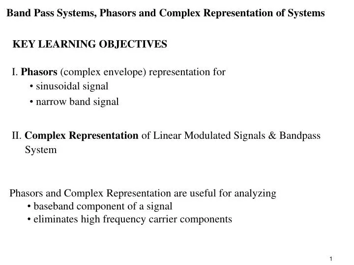
Band Pass Systems, Phasors and Complex Representation of Systems KEY LEARNING OBJECTIVES • I. Phasors (complex envelope) representation for • sinusoidal signal • narrow band signal • II. Complex Representation of Linear Modulated Signals & Bandpass • System • Phasors and Complex Representation are useful for analyzing • baseband component of a signal • eliminates high frequency carrier components
2W X(f) -f0 -W -f0 - f0 +W f0 -W f0 f0 +W • h(t) is aBandpass System,, that passes signals with frequency components in • the neighborhood of some frequency, f0 • H(f)= 1 for | f – f0 | ≤ W otherwise H(f)≈ 0 • bandpass system h(t) passes a bandpass signal x(t) X(f) X(f) H(f) I. Phasors for monochromatic & narrow band signals • x(t) is a narrowband signal (aka bandpass signal) if • X(f) ≠ 0 in some small neighborhood of f0 ,a high frequency • X(f)≡ 0 for | f – f0 | ≥ W where W < f0 • f0is usually referred to as center frequency, but need not be • center frequency or in signal bandwidth at all
Consider LTI system driven by input x(t) H(f) Y(f) X(f) • output determined by multiplying X & frequency response of • system computed at input frequency, f0 • input & output frequencies are same output phasor gives output • signal • determine the phasor for sinusoida1 signal and narrowband signal • capture phase and magnitude of base band signal • ignore effects of the carrier
I Aexp(jθ) xq(t) 2πf0 R x(t) 1. determination of phasor,X for sinusoidal input signal x(t) • x(t) = Acos(2πf0 t + θ) • xq(t) =Asin(2πf0 t + θ) • quadrature component shifted 90o from x(t) (i) define a signal z(t) as a vector rotating with angular frequency 2πf0 z(t) = Aexp(j(2πf0t + θ)) = Acos(2πf0t + θ) + jAsin(2πf0t + θ) = x(t) + jxq(t) • (ii) obtain phasorX from z(t) by eliminating 2πf0 rotation • - rotate z(t) at an angular frequency = 2πf0 in opposite direction • - equivalent to multiplying z(t) by exp(2πf0t) • X = z(t) exp(-j2πf0t ) = Aexp(j(2πf0t + θ))exp(-j2πf0t ) • = Aexp(jθ)
x(t) = Acos(2πf0t + θ) = Acos(θ)cos(2πf0t)+ Asin(θ)sin(2πf0t) sin(θ)[δ(f+f0) - δ(f-f0)] X(f) = cos(θ)[δ(f–f0 ) + δ(f+f0)] - j [cos(θ)δ(f–f0 ) + jsin(θ)δ(f–f0 )] Z(f) = (2) determine Z(f) = F[z(t)] z(t) = Aexp(j(2πf0t + θ)) = Aexp(jθ)exp(j2πf0t ) since F[exp(j2παt)] = {δ(f-α)} Z(f) = Aexp(jθ)δ(f – f0 ) (ii) then shift Z(f) by f0 X = Aexp(jθ) 1a. determine Frequency Domain equivalent of z(t) and X (i) obtain Z(f), using either or two methods (1) determine X(f) = F[x(t)], delete negative frequencies & multiply by 2
2. determine phasor for a narrowband signal, x(t) based on definition of z(t) in sinusoid case: z(t) = x(t) + jxq(t) find Z(f) by deleting negative frequencies of X(f) & multiply result by 2 Z(f) = 2u-1(f)X(f) z(t) = we know that F[u-1(t)] = by duality = u-1(f) by convolution let then z(t) = z(t) is known as theanalytic signal or pre-envelope of x(t) • find z(t) using IFT find signal whose Fourier transform = u-1(f)
(i) sinusoid case z(t) x(t) = Acos(2πf0 t+θ) xq(t)= Asin(2πf0 t+θ) = x(t) + jxq(t) z(t)= x(t) + j (ii) narrowband case phase shift x(t) by for positive frequencies phase shift x(t) by for negative frequencies Hilbert Transform of x(t) is given by pre-envelope for two types of signals
determine phasor, xl(t)of bandpass signal x(t) • xl(t) = low pass representation of x(t) • determined by shifting spectrum of z(t) left by f0 A X(f) f Z(f) 2A f0 f0 f f0 Xl(f) 2A f Xl(f) = Z(f + f0) = 2u-1(f + f0)X(f + f0) xl(t) = z(t)exp(-j2πf0t) • xl(t)is a low pass signal • Xl(f)≡ 0 for all | f | ≥ W • phasor for band pass signal
ˆ x ( t ) rewrite in terms of quadrature & in-phase components z(t)= • z(t) = xl(t)exp(j2πf0t) • = [xc(t) + jxs(t)]exp(j2πf0t) • = xc(t)cos(2πf0t) - xs(t)sin(2πf0t) + j[xc(t)sin(2πf0t)+xs(t)cos(2πf0t)] equate real & imaginary parts of z(t) and xl(t) ˆ x ( t ) x(t) = Re{z(t)} = xc(t)cos(2πf0t) - xs(t)sin(2πf0t) = Im{z(t)} = xc(t)sin(2πf0t)+xs(t)cos(2πf0t) Generallyxl(t)is complex signal with real (in phase) & imaginary (quadrature) components xl(t) = xc(t) + jxs(t) bandpass to lowpass transform describes relationship of x(t) & in terms of xc(t)&xs(t)
define envelope of xl(t) as V(t) = define phase of xl(t) as I Θ(t) = xl(t) then xl(t) = V(t)exp( jΘ(t) ) V(t) = Θ(t) R V(t) & Θ(t) are slowly time varying • monochromatic phasor has constant amplitude & phase • bandpass signal’s phase & envelope vary slowly with time vector • representation moves on a curve in the complex plane Define xl(t) in terms of phase & envelope
II. Complex Representation of Linear Modulated Signals & Bandpass System canonical representation of anybandpass signal, s(t) has 2 components s(t) = sI(t)cos(2πfct) - sQ(t)sin(2πfct) • sI(t) = in-phase component of s(t) • sQ(t) = quadrature component of s(t) • properties of sI(t) & sQ(t) • are real valued functions • are orthogonal to each other • are uniquely defined in terms of the baseband signalm(t) • two components can be used to synthesize modulated signals(t)
circuit used to synthesizes(t) from sI(t) & sQ(t) sI(t) sQ(t) cos(2fct) s(t) oscillator 90o sin(2fct) circuits used to analyzesI(t) & sQ(t)based on s(t), sI(t) LPF 2cos(2fct) oscillator s(t) 90o -2sin(2fct) sQ(t) LPF
1. Complex Envelope ofa Band-Pass Signals(t) is given as s̃̃(t) = sI(t) + jsQ(t) s̃̃(t) preserves information content of s(t), except for fc(t) • s̃̃(t)e(2πfct)= [sI(t) + jsQ(t)] [cos(2πfct) + jsin(2πfct)] • = sI(t)cos(2πfct) - sQ(t)sin(2πfct) + j[sI(t)sin(2πfct)+sQ(t)cos(2πfct)] real imag then, • s(t) = Re{s̃̃(t)e(2πfct)} • = sI(t)cos(2πfct) - sQ(t)sin(2πfct)
x(t) h(t) y(t) x̃̃(t) h̃̃(t) 2ỹ(t) 2. Consider a narrowband linear band-pass system • system is narrowband if bandwidth W << fc, the system’s center • frequency • input x(t) is modulated by carrier, fc • output = y(t) canonical representation of system’s impulse response given by: h(t) =hI(t)cos(2πfct) - hQ(t)sin(2πfct) use equivalent complex baseband model to simplify analysis • impulse response given by h̃̃(t) = hI(t) + jhQ(t)
y(t) = [xI()cos(2πfc )-xQ(t)sin(2πfc )]· [hI(t-)cos(2πfct-)-hQ(t-)sin(2πfct-)]d y(t) = = xI(t) hI(t-) cos(2πfct)cos(2πfct-)d + xQ(t) hQ(t-) sin(2πfct)sin(2πfct-)d - xI(t)hQ(t-)cos(2πfct)sin(2πfct-) d - xQ(t)hI(t-)cos(2πfct-)sin(2πfct) d 2.1 Passband Analysis of LTI System
y(t) + xQ(t) hQ(t-) ½[ cos() - cos(4πfc t-) ] d = xI(t) hI(t-) ½[ cos() + cos(4πfc t-) ] d - - xI(t)hQ(t-)½[ sin(4πfc t) + sin() ] d xQ(t)hI(t-)½[ sin(4πfc t) - sin() ] d Passband Analysis of LTI System (continued)
complex input & output are complex envelopes of bandpass systems • input & output x̃̃(t)= xI(t) + jxQ(t) is the complex envelope of x(t) ỹ(t) = yI(t) + jyQ(t) is the complex envelope of y(t) ỹ(t) = = 2.2 Equivalent Complex Baseband Model • complex envelopes are related by complex convolution = [xI(t) + jxQ(t)][hI(t-λ) + jhQ(t-λ)]dλ = hI(t-λ)xI(t) - hQ(t-λ)xQ(t) + j[xQ(t)hI(t-λ) + hQ(t-λ)xI(t)]dλ
Passband signalsare readily determined from ỹ(t) and x̃̃(t) x(t) = Re{x̃̃(t)exp(2πfct)} y(t) = Re{ỹ(t)exp(2πfct)} Impulse response of band-pass system given by h(t) = Re{h̃̃(t)exp(2πfct)} = Re{ (hI(t) + jhQ(t))(cos(2πfct) + jsin(2πfct) )} = hI(t)cos(2πfct) - hQ(t) sin(2πfct) Equivalent Notation for complex baseband model ( ‘’ = convolution) ỹ(t) =½(x̃̃(t)h̃̃(t)) = ½(h̃̃(t) x̃̃(t)) • ½ factor added to maintain equivalence between real & complex models • fcis omitted from complex baseband model simplifies analysis • without loss of information
phasor representing phase & magnitude of x(t) = complex envelope: x exp(jx) = xcos(x) + jx sin(x) x = magnitude x = argument (phase of x(t)) Appendix: More on Complex Envelope - viewed as an extension of phasor for a real harmonic signal x(t) x(t) = x cos(2f0t + x) t R • assume x 0 and phase is 0 x < 2, then: (i) exp(j(2f0t+x )) = cos(2f0t +x) + jsin(2f0t +x) (ii) x(t) = Re[x( cos(2f0t +x) + jsin(2f0t +x) )] t R = Re [x exp(j(2f0t + x))] t R = Re [x exp(jx)exp(j2f0t )] t R
derive complex envelope for any real continuous signal, x(t) assumex(t) = Re [xe(t)exp(j2f0t )] t R where xe(t)= x exp(jx), X(f) = F[xcos(2f0t+ x)] = xexp(jx)(f-f0) + xexp(-jx)(f+f0) = xexp(jx)(f-f0) f R x̃̃p(f) = xe(t) = xexp(jx) F-1[x̃̃e(f) ] i. Take Fourier Transform of x(t) ii. suppress negative frequencies & multiply by 2 iii. shift left by f0to obtain frequency signal x̃̃e(f) = xexp(jx)(f0) f R iv. take Inverse Fourier Transform
e.g. Pure Harmonic signal given by x(t) = cos(2f1t + x) t R = exp(j)(f-f1) x̃̃p(f) x̃̃e(f) = exp(j)(f-f1+f0) • where x 0 • 0 x < 2 i. FT yields X(f) = ½ exp(jx)(f-f1) + ½ exp(-jx)(f+f1) ii. iii. iv xe(t) = exp(j)exp(2j(f1-f0))t t R • if f1 = f0 complex envelope = phasor • if |f1-f0| << f0 xe varies slowly compared to exp(2jf0t)
If x(t) = real, continuous function, & F(x) has no delta function at f = 0 pre-envelope (aka analytical) of x is complex valued signal xp with complex-envelope of x with respect to frequency f0 is signal xe F[x̃̃p]= x̃̃p(f) = 2X(f)1(f) f R x̃̃e(f) = x̃̃p(f+f0) = 2X(f+f0) 1(f+f0) f R xe(t)= F-1[ x̃̃e(f)]
Complex Envelope for let x(t) = real, band-pass, band-limitedsignal • fc = center frequency & W = bandwidth • where W < fc, are positive real numbers (W << fc x(t) is narrowband) • X(f) = 0 for | f | < fc-W and | f | > fc+W f R X(f) W W 0 -fc 0 fc ˆ x ( f ) p 0 fc • xe = complex envelope with respect to f0 • contains only low frequencies • f0 R+ xeis not uniquely defined 0 xp = analytical