Download
1 / 13
140 likes | 457 Views
Left – Lord Rayleigh, pronounced like Riley. He was a famous physicist who, among other things, discovered Argon and explained why the sky was blue. And, it still is!. The Rayleigh Model. Kan Ch 7 Steve Chenoweth, RHIT. It’s a Weibull distribution…. Used in physics:

E N D
Left – Lord Rayleigh, pronounced like Riley. He was a famous physicist who, among other things, discovered Argon and explained why the sky was blue. And, it still is! The Rayleigh Model KanCh 7 Steve Chenoweth, RHIT
It’s a Weibull distribution… • Used in physics: • It’s “Rayleigh” when m = 2.
The Rayleigh Model is widely used • Lots of applications other than possibly the distribution of software bugs. • E.g., it’s what you get when two uncorrelated random variables combine. m = 2 Big batch of Weibulls Probability density function (PDF) Cumulative distribution function (CDF)
So, for Rayleigh… • We have this, • Where t = time and c = the “scale parameter,” and is a function of tm, the time at which the curve reaches its peak. (Set the derivative of f(t) = 0 to get:
For software • Projects follow a life-cycle pattern described by the Rayleigh density curve. • Used for: • Staffing estimation over time • Defect removal pattern – expected latent defects
Assumes… • Defect removal effectiveness remains relatively unchanged. Then – • Higher defect rates in development are indicative of higher error injection, and • It is likely that the field defect rate will also be higher. • Given the same error injection rate, if more defects are discovered and removed earlier, fewer will remain in later stages. Then – • Field quality will be better.
Kan studied this • A formal hypothesis-testing study, based on component data of the AS/400. • Strongly supported his first assumption. • Found proving the second assumption trickier.
Implementation • Kan says it’s “not difficult.” • Adds elsewhere, “if you have an SAS expert handy.” • If defect data (counts or rates) are reliable, • Model parameters can be derived, then • Just substitute data values into the model. • Also built into software tools like SLIM (see p 200).
Reliability • Can judge by testing “confidence interval.” • Which relates to sample size. • Kan recommends – use multiple models, to cross-check results.
Validity • Depends heavily on “data quality” • Which is notoriously low related to software • Usually better at back-end (testing) • And, “Model estimates and actual outcomes must be compared and empirical validity must be established.” • In our current state of the art, validity and reliability are “context specific.”
In Kan’s study… Rayleigh underestimated the tail!