Download
1 / 10
110 likes | 388 Views
Enrollment Forecasting with ARIMA Time-Series Modeling. Jamie DeLeeuw, Ph.D. Monroe County Community College MI AIR 2013. Do tuition and/or unemployment rate predict enrollment (headcount, credit hours, billable contact hours)? . Previous Studies.

E N D
Enrollment Forecasting with ARIMA Time-Series Modeling Jamie DeLeeuw, Ph.D. Monroe County Community College MI AIR 2013
Do tuition and/or unemployment rate predict enrollment (headcount, credit hours, billable contact hours)?
Previous Studies • Student Price Response Coefficient (SPRC): The percentage change in enrollment given a fixed tuition increase per year. • Controlling for unemployment rate and need-based grant spending per state, Kane (1995) found that a $1000 tuition increase (1991 dollars) led to a 3.5% decrease in enrollment at community colleges (CC’s) and a 1.4% decline at four-year institutions. • CC’s: Controlling for unemployment rate and need-based grant spending, an increase of $100 (1993 dollars) resulted in a .33% decrease in enrollment (Heller, 1996, as cited in Heller, 1997). • Tuition elasticity: The percentage change in enrollment given a percentage change in tuition. • A tuition increase of 8% led to a 0.9% decrease in CC enrollment (Rouse, 1994) . • The demand price elasticity of California CC’s was -0.15 (Shires, 1995).
Previous Studies • Slight inverse relationship between tuition & enrollment, as evidenced in Heller’s (1997) meta-analysis as well as the aforementioned studies; others have found either the opposite effect or no effect (Craft, Baker, Myers, & Harraf, 2012; Shin and Milton, 2008). • Unemployment and enrollment: Most demonstrate no relationship between the variables (Craft et al., 2012; Hemelt & Marcotte, 2011, Stanley & French, 2009). Kane (1995) however found that 2-year public college enrollment was positively related to unemployment, whereas 4-year institutions’ enrollment was inversely related.
Limitations to Prior Research:Gallet’s (2007) Meta-Analysis • A majority (72.5%) of tuition analyses use ordinary least squares (OLS). This method is problematic in that OLS assumes homoscedasticity and lack of autocorrelation in the residuals (Tabachnick & Fidell, 2007). • Regardless of the procedure used, analyses have tended to cover the short-run (91%) and correction for autocorrelation (28%), heteroscedasticity (7%), and multicollinearity (11%) has been rare. • In studies that include adjustments for autocorrelation and heteroscedasticity, enrollment is less affected by tuition increases. ______________________________________________ • Previous research tends to conglomerate data from multiple institutions and assesses Fall (typically full-time) headcount fluctuations over a limited time span.
ARIMA • Autoregressive Integrated Moving Average (ARIMA) time-series analysis is an ideal way to examine enrollment patterns over time, test whether variables serve as predictors, and forecast future enrollment, while avoiding the aforementioned statistical blunders. • A model (p, d, q)(P, D, Q) is selected that best characterizes patterns in the data: p = auto-regression d = integrated (linear or quadratic trend)…differencing or transformation? q = moving average (random shocks)
Goodness-of-Fit • Ljung-Box statistic: Whether model is correctly specified; desire > .05 • Stationary R²: Estimate of the proportion of the total variation in the series that is explained by the model; more appropriate than ordinary R² when there is trend or a seasonal pattern • Model outliers? • Are predictors statistically significant? • Graphs • ARIMA Expert Modeler vs. playing around
Getting the Data Ready • Tuition: Credit hour + technology fee • U.S. Inflation Calculator (converted $ to 2011) • County Unemployment Rate: • http://data.bls.gov/map/MapToolServlet?survey=la • 50+ data points • Enrollment (DV): Headcount, credit hour, billable contact hour • Credit to contact hour conversion if needed • Define dates • Reminder: If your model contains significant predictors, those need to be forecasted or entered before forecasting the DV(enrollment)
Results • Using FA, WI, SP, & SU data from Fall 2002 to Fall 2013, 96.3% of the total variation in billable contact hours was captured by the model. Neither county unemployment rate nor tuition served as enrollment predictors. We can be 95% confident that Winter 2014 contact hour enrollment will lie somewhere between 33542 and 40413, with the best estimate being 36977. It is important that new data be added each semester to capture recent policy changes and trends, thereby increasing the accuracy of the forecast. • The following may avert enrollment declines when tuition increases (Leslie and Brinkman,1987; Shin & Milton, 2008): • Low tuition relative to other CC’s in the region • Habituation to small increases…and other institutions increase as well • Perceived higher demand for payoff (?) • Enhanced marketing (?) • Increased access for minority and non-traditional students • IPEDS data indicate FTIACs who received federal grant aid at this institution increased from 19% in 2002 to 40% in 2009; the average amount increased from $3228 to $4462.
References Craft, R. K., Baker, J. G., Myers, B. E., & Harraf, A. (2012). Tuition revenues and enrollment demand: The case of southern Utah university (Professional File No. 124). Gallet, C. (2007). A comparative analysis of the demand for higher education: Results from a meta-analysis of elasticities. Economics Bulletin, 9(7), 1-14. Heller, D. E. (1997). Student price response in higher education: An update to Leslie and Brinkman. The Journal of Higher Education, 68(6), 624-659. Hemelt, S. W., & Marcotte, D. E. (2011). The impact of tuition increases on enrollment at public colleges and universities. Educational Evaluation and Policy Analysis, 33(4), 435-457. IBM SPSS Forecasting 19 Kane, T. J. (1995). Rising public college tuition and college entry: How well do public subsidies promote access to college (Working Paper No. 5164). Leslie, L. L., and Brinkman, P. T. (1987). Student price response in higher education. Journal of Higher Education, 58, 181-204. Rouse, C. E. (1994). What to do after high school: The two-year versus four-year college enrollment decision. In R. G. Ehrenberg (Ed.), Choices and consequences: Contemporary policy issues in education (pp. 59-88). Ithaca, NY: ILR Press. Shin, J. C., & Milton, S. (2008). Student response to tuition increase by academic majors: Empirical grounds for a cost-related tuition policy. Higher Education, 55, 719-734. Shires, M.A. (1996). The future of public undergraduate education in California. Santa Monica,CA: RAND Institute. Stanley, R. E., & French, P. E. (2009). Evaluating increased enrollment levels in institutions of higher education: A look at merit-based scholarship program. Public Administration Quarterly, 33(1), 4-36. Tabachnick, B.G., & Fidell, L.S. (2007). Using multivariate statistics (5th ed.). Boston, MA: Allyn & Bacon.