Download
1 / 15
290 likes | 680 Views
Time Series and Forecasting. Chapter 16. Goals. Define the components of a time series Compute moving average Determine a linear trend equation Compute a trend equation for a nonlinear trend

E N D
Time Series and Forecasting Chapter 16
Goals • Define the components of a time series • Compute moving average • Determine a linear trend equation • Compute a trend equation for a nonlinear trend • Use a trend equation to forecast future time periods and to develop seasonally adjusted forecasts • Determine and interpret a set of seasonal indexes • Deseasonalize data using a seasonal index • Test for autocorrelation
Time Series and its Components • TIME SERIES is a collection of data recorded over a period of time (weekly, monthly, quarterly), an analysis of history, that can be used by management to make current decisions and plans based on long-term forecasting. It usually assumes past pattern to continue into the future • Components of a Time Series • Secular Trend – the smooth long term direction of a time series • Cyclical Variation – the rise and fall of a time series over periods longer than one year • Seasonal Variation – Patterns of change in a time series within a year which tends to repeat each year • Irregular Variation – classified into: • Episodic – unpredictable but identifiable • Residual – also called chance fluctuation and unidentifiable
The Moving Average Method • Useful in smoothing time series to see its trend • Basic method used in measuring seasonal fluctuation • Applicable when time series follows fairly linear trend that have definite rhythmic pattern
Weighted Moving Average • A simple moving average assigns the sameweight to each observation in averaging • Weighted moving average assigns differentweights to each observation • Most recent observation receives the most weight, and the weight decreases for older data values • In either case, the sum of the weights = 1 Cedar Fair operates seven amusement parks and five separately gated water parks. Its combined attendance (in thousands) for the last 12 years is given in the following table. A partner asks you to study the trend in attendance. Compute a three-year moving average and a three-year weighted moving average with weights of 0.2, 0.3, and 0.5 for successive years.
Linear Trend • The long term trend of many business series often approximates a straight line • Use the least squares method in Simple Linear Regression (Chapter 13) to find the best linear relationship between 2 variables • Code time (t) and use it as the independent variable • E.g. let t be 1 for the first year, 2 for the second, and so on (if data are annual)
The sales of Jensen Foods, a small grocery chain located in southwest Texas, since 2005 are: Linear Trend – Using the Least Squares Method: An Example
Nonlinear Trends • A linear trend equation is used when the data are increasing (or decreasing) by equal amounts • A nonlinear trend equation is used when the data are increasing (or decreasing) by increasing amounts over time • When data increase (or decrease) by equal percents or proportions plot will show curvilinear pattern • Top graph is original data • Graph on bottom right is the log base 10 of the original data which now is linear (Excel function: Y = log(x) or log(x,10) • Using Data Analysis in Excel, generate the linear equation • Regression output shown in next slide
Seasonal Variation and Seasonal Index • One of the components of a time series • Seasonal variations are fluctuations that coincide with certain seasons and are repeated year after year • Understanding seasonal fluctuations help plan for sufficient goods and materials on hand to meet varying seasonal demand • Analysis of seasonal fluctuations over a period of years help in evaluating current sales SEASONAL INDEX • A number, usually expressed in percent, that expresses the relative value of a season with respect to the average for the year (100%) • Ratio-to-moving-average method • The method most commonly used to compute the typical seasonal pattern • It eliminates the trend (T), cyclical (C), and irregular (I) components from the time series
Seasonal Index – An Example EXAMPLE The table below shows the quarterly sales for Toys International for the years 2001 through 2006. The sales are reported in millions of dollars. Determine a quarterly seasonal index using the ratio-to-moving-average method. Step (1) – Organize time series data in column form Step (2) Compute the 4-quarter moving totals Step (3) Compute the 4-quarter moving averages Step (4) Compute the centered moving averages by getting the average of two 4-quarter moving averages Step (5) Compute ratio by dividing actual sales by the centered moving averages
Actual versus Deseasonalized Sales for Toys International Deseasonalized Sales = Sales / Seasonal Index
Seasonal Index – An Example Using Excel Given the deseasonalized linear equation for Toys International sales as Ŷ=8.109 + 0.0899t, generate the seasonally adjusted forecast for each of the quarters of 2010 Ŷ X SI = 10.62648 X 1.519 Ŷ = 8.10 + 0.0899(28)