Download
1 / 24
480 likes | 1.53k Views
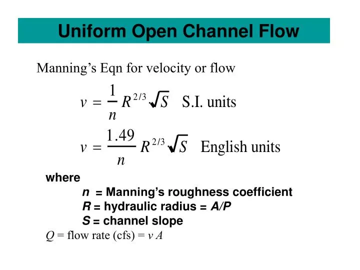
Uniform Open Channel Flow . Manning’s Eqn for velocity or flow. where n = Manning’s roughness coefficient R = hydraulic radius = A/P S = channel slope Q = flow rate (cfs) = v A. Uniform Open Channel Flow – Brays B. Brays Bayou. Concrete Channel.

E N D
Uniform Open Channel Flow Manning’s Eqn for velocity or flow where n = Manning’s roughness coefficient R = hydraulic radius = A/P S = channel slope Q = flow rate (cfs) = v A
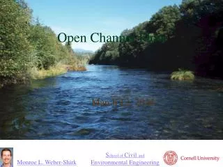
Uniform Open Channel Flow – Brays B. Brays Bayou Concrete Channel
Normal depth is function of flow rate, and geometry and slope. Can solve for flow rate if depth and geometry are known. • Critical depth is used to characterize channel flows -- based on addressing specific energy: • E = y + Q2/2gA2 where Q/A = q/y • Take dE/dy = (1 – q2/gy3) = 0. • For a rectangular channel bottom width b, • 1. Emin = 3/2Yc for critical depth y = yc • yc/2 = Vc2/2g • yc = (Q2/gb2)1/3
Critical Flow in Open Channels • In general for any channel, B = top width • (Q2/g) = (A3/B) at y = yc • Finally Fr = V/(gy)1/2 = Froude No. • Fr = 1 for critical flow • Fr < 1 for subcritical flow • Fr > 1 for supercritical flow
Non-Uniform Open Channel Flow With natural or man-made channels, the shape, size, and slope may vary along the stream length, x. In addition, velocity and flow rate may also vary with x. Thus, Where H = total energy head z = elevation head, v2/2g = velocity head
Replace terms for various values of S and So. Let v = q/y = flow/unit width - solve for dy/dx
Given the Fr number, we can solve for the slope of the water surface - dy/dx Note that the eqn blows up when Fr = 1 or So = S where S = total energy slope So = bed slope, dy/dx = water surface slope
Now apply Energy Eqn. for a reach of length L This Eqn is the basis for the Standard Step Method to compute water surface profiles in open channels
Routine Backwater Calculations Select Y1 (starting depth) Calculate A1 (cross sectional area) Calculate P1 (wetted perimeter) Calculate R1 = A1/P1 Calculate V1 = Q1/A1 Select Y2 (ending depth) Calculate A2 Calculate P2 Calculate R2 = A2/P2 Calculate V2 = Q2/A2
Backwater Calculations (cont’d) Prepare a table of values Calculate Vm = (V1 + V2) / 2 Calculate Rm = (R1 + R2) / 2 Calculate Manning’s Calculate L = ∆X from first equation X = ∑∆Xi for each stream reach (SEE SPREADSHEET)
Watershed Hydraulics Bridge D QD Tributary Floodplain C QC Main Stream Bridge Section B QB A QA Cross Sections Cross Sections
Brays Bayou-Typical Urban System • Bridges cause unique problems in hydraulics • Piers, low chords, and top of road is considered • Expansion/contraction can cause hydraulic losses • Several cross sections are needed for a bridge • Critical in urban settings 288 Crossing
The Floodplain Top Width
The Woodlands • The Woodlands planners wanted to design the community to withstand a 100-year storm. • In doing this, they would attempt to minimize any changes to the existing, undeveloped floodplain as development proceeded through time.