Download
1 / 52
590 likes | 932 Views
OPEN CHANNEL FLOW. Basic terms in study of open channel flow are: discharge or cross-sectional area A , wetted perimeter O , hydraulic radius R h = A / O and volume discharge Q . For the rectangular cross-section: (for “real” river h / B 0 ; R h = h ).

E N D
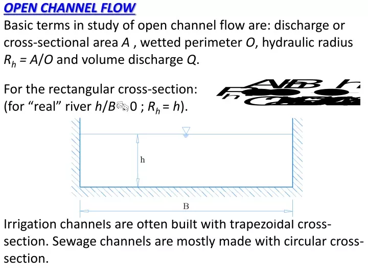
OPEN CHANNEL FLOW Basic terms in study of open channel flow are: discharge or cross-sectional areaA , wetted perimeter O, hydraulic radius Rh = A/O and volume discharge Q. For the rectangular cross-section: (for“real” river h/B0 ; Rh = h). Irrigation channels are often built with trapezoidal cross-section. Sewage channels are mostly made with circular cross-section.
OPEN CHANNEL FLOW Partially regulated channels often occur as composite channels. Natural riverbeds are nonuniform. The depth is defined as vertical distance between the free surface and the lowest point on the line of cross section. If the bed is made of resistant material the profile will remain stable and unchanged over time. Otherwise, erosion and deposition will lead to a meandering process. Man-made regulation (inundation + dike) Nature main river bad
OPEN CHANNEL FLOW Classification for open channel flow: uniform and nonuniform Classification for open channel flow: steady - unsteady
OPEN CHANNEL FLOW laminar and turbulent Critical Reynolds number for open channel flow D = 4RhRekrit 500 subcritical, critical and supercritical
OPEN CHANNEL FLOW – resistance and turbulen flow For the practical purposes one can adopt the logarithmic velocity profile along the vertical: It is a non-dimensional equation that relates velocity u in particular point of vertical axes, mean velocity V and “shear velocity” u*. The channel bed with higher roughness induces more intense turbulence. That will cause a decrease in near-bottom velocities, as well asan increase in free surface velocity. Using the logarithmic velocity profile, Koriolis kinetic energy coefficient has the value 1,04.
OPEN CHANNEL FLOW – resistance and turbulen flow The distribution of shear stresses along the contour of trapezoidal cross-section is given in the figure: The consequence of non-uniform stress distribution is the onset of „weak“ secondary flow in cross section and shift of maximum velocity position from the surface to the deeper layer.
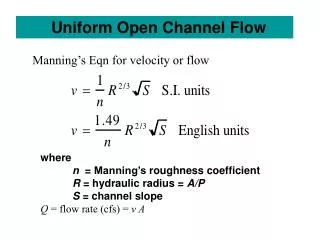
OPEN CHANNEL FLOW – uniform flow The first task in engineering practice is to calculate the cross-section average velocity V and volume discharge Q for an arbitrary cross-section A. In the case of uniform flow Chezy equation is commonly used: C - Chezy roughness coefficient I0 – slope of channel bottom For the uniform flow condition: I0 = IPL= IEL IPL – slope of piezometric line (slope of free surface) IEL – slope of energy line IEL To define Chezy‘s roughness coefficient in practice is frequently used Manning's coefficient of roughness n:
OPEN CHANNEL FLOW – uniform flow For uniform and stationary flow conditions Chezy equation would define the relation Q(h) = V(h)*A(h) or so-called “consumption curve”.
OPEN CHANNEL FLOW – local changes in cross-section geometry The occurrence of “sudden” changes in channel geometry causes gradually changes in the flow geometry. The disturbances of free surface are present “upstream” and “downstream” from the position of change. Intensified vorticity in the vicinity of geometry disturbance is responsible for the “local” losses of mechanical energy: V – average velocity in flow cross-section
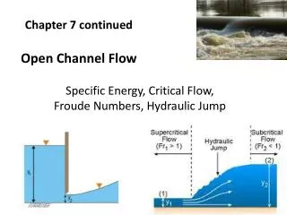
OPEN CHANNEL FLOW – cross-section specific energy The flow through an arbitrary cross-section can be also divided according to the gravity participation in the overall inertia force. The appropriate regimes are termed as: subcritical, critical or supercritical. We need to introduce the idea of specific energyE of cross-section that is defined by equation: In order to yield the extrema of specific energy function E we apply the first derivate: dA = BdhFroude number (**2)
OPEN CHANNEL FLOW – cross-section specific energy Fr < 1 subcritical Fr > 1 supercritical Fr = 1 critical The depth at which Fr = 1 one terms as critical depth hkr and associated cross-section average velocity as critical velocity vkr. If discharge Q and specific energy E are fixed (Q, E = const.), two solutions for h arise from above equation (h1 and h2). Those two depths approach each other when decreasing the specific energy E. At minimum specific energy E = Emin only one depth can exist and that is the critical depth hkr (Fr2 = Fr =1) Critical depth hkr for rectangular cross-section is obtained explicitly: (q = hkr*Vkr)
OPEN CHANNEL FLOW – cross-section specific energy Specific energy diagram (specific energy curve for cross-section) (specific energy E is the function of depth h under the constant specific discharge q) h>hkr(Fr < 1) subcritical condition h<hkr(Fr > 1) supercritical condition IMPORTANT: One curve is obtained by fixed Q (or q)and varying the channel bed slope I
OPEN CHANNEL FLOW – cross-section specific energy For any available specific energy E exists the corresponding maximum discharge qmax that is “transported” at critical condition (hkr and Vkr). Example: the flow over a submerged hump .
OPEN CHANNEL FLOW – cross-section specific energy Flows in open channels will overcome the “obstacles” (weirs) on “economic” way, achieving the critical depth in the vicinity of the structure crest (highest datum-level). Flow regime upstream of the obstacle is subcritical, on the weir profile or over the submerged wide weir is critical, and downstream of obstacle depends on channel bottom slope (I0<Ikrit , h>hkr, Fr < 1 subcritical I0>Ikrit , h<hkr, Fr > 1 supercritical).
OPEN CHANNEL FLOW – cross-section specific energy Let us apply the idea of specific energy to the example of steady flow under the plate with the neglected lines and local losses. The depths before and after the plate (h1, h2) are related to the same specific discharge q and specific energy E.
OPEN CHANNEL FLOW – cross-section specific energy Raising the plate above the critical depth hkr results in maximum possible discharge qmax for the available specific energy E.
OPEN CHANNEL FLOW – cross-section specific energy Flow above the hump with relatively “low” denivelation h (we assume neglected energy losses). subcritical supercritical
OPEN CHANNEL FLOW – overflow and underflow Flow over sharp-crested weir P is the weir height, B is channel width, h0 is incoming depth andV0 is average cross section incoming velocity in subcritical regime of flow. Energy losses are to be neglected. Above the highest weir datum one would find the critical depth : hp - overflowing depth (vertical distance from weir crest to the free surface at distance of 4hp from the weir cross section).
OPEN CHANNEL FLOW – overflow and underflow Considering the critical condition over the weir crest the overflowing discharge can be calculated applying the equation: After a few steps of editing the above equation one gets: CQ - nondimensional discharge coefficient In case of “high” weir hp/P0 ; V00: The above equation is also used for the other types of weirs. The value of discharge coefficient CQ is obtained experimentally. Generally, discharge coefficient CQ depends on:
OPEN CHANNEL FLOW – overflow and underflow More common used form is the ogee weir or ogee spillway with the rounded crest :
OPEN CHANNEL FLOW – overflow and underflow Underflow At a sufficient upstream distance from the gate (plate) the streamlines are parallel and the pressure distribution along the water column is hydrostatic.
OPEN CHANNEL FLOW – overflow and underflow The flow is pronouncedly nonuniform in gate cross-section (streamlines are not parallel). At a certain downstream distance from the gate appears another cross-section with parallel streamlines, so-called contraction cross-section. The ratio between the gate opening height “s” and contracted depth h1 is termed as contraction coefficient CC (obtained experimentally ; h1 = CC s).
OPEN CHANNEL FLOW – overflow and underflow For the flow under the gate of width B following equality are valid: - contraction cross-section area A1=CC s B • continuity equation Q0=Bh0V0 = Q1= BCC sV1 • specific energy is equal for the both of cross-sections E0 = E1 (energy losses are neglected) In case of horizontal bottom and great upstream depth s/h00 ; Fr0 0 the discharge coefficient reads CQ = 0,611.
OPEN CHANNEL FLOW – hydraulic jump The transition from supercritical to subcritical flow regime is related to the hydraulic phenomena called hydraulic jump. Rapid decrease in average velocity and increase of depth, including the high degree of mechanic energy loss takes place in the hydraulic jump. Because of energy loss hv , the concept of specific energy is no longer valid and applicable (energy loss in hydraulic jump is not apriori known). Normal hydraulic jump
OPEN CHANNEL FLOW – hydraulic jump We can use the law of momentum conservation and apply it on the control volume that include normal hydraulic jump. q =V1h1=V2h2 h1,h2- first and second conjugate depth - averaged tangential stresses at the bottom Lj - length of hydraulic jump MemberLj is negligible in comparison to the pressure force. Normal hydraulic jump
OPEN CHANNEL FLOW – hydraulic jump Applying the momentum and continuity equations one defines the relationship between the conjugate depths h1 i h2: Fr1 - Froude number in cross section where h1 After the calculation of h2 and V2 , one can find the intensity of energy loss (dissipation) within the hydraulic jump by :
OPEN CHANNEL FLOW – hydraulic jump The length of hydraulic jump is to be determined experimentally. For the practical purpose one can use relation Lj 6,1h2. Increase of Fr1 causes the decrease of h2/h1 and hv/E1. If downstream normal depth h is greater then second conjugate depth h2, hydraulic jump will occur in so-called submerged form. Conversely, hydraulic jump will occur in so-called thrown form that can threat the bottom stability.
OPEN CHANNEL FLOW – hydraulic jump If submerged condition is not assured, one has to carry out the so-called stilling basin. Stilling basin provides the stabilization (localization) of hydraulic jump within its geometry. Stilling basin is carried out after the spillway, excavating the cave below the level of natural river bottom.
GROUNDWATER FLOW IN POROUS MEDIA Darcy velocity v = Q/A applies primarily in the analysis of groundwater flow (flow in porous underground aquifers). It relies on the assumption of the continuum (v = Q/A ) where the presence of the solid phase within the flow cross-section A is not taken into account. “Real” velocity is higher then Darcy velocity, what is especially important in the analysis of pollution transport in aquifers.
GROUNDWATER FLOW IN POROUS MEDIA Darcy experimental device is used for determine the Darcy filtration coefficient (hydraulic conductivity) k of particular filter material. It is obtained by measuring the Darcy velocity as v = Q/A and pezometric slope I = h/l (ratio of piezometric drop h on path length l ).
GROUNDWATER FLOW IN POROUS MEDIA In general 3D case k is the tensor dependent on geological strata and flowing liquid. Groundwater flow can be observed as potential flow.
GROUNDWATER FLOW IN POROUS MEDIA In potential flow the flow field is defined with flow mesh that consists of equipotentials and streamlines.
GROUNDWATER FLOW IN POROUS MEDIA Hydraulic (Dupuit) flow theory neglects the vertical component of flow velocity (equipotentials are vertical lines). Vertical component of the flow can not be ignored in the vicinity of the well (strong deviation from Dipuit assumption).
GROUNDWATER FLOW IN POROUS MEDIA Aquifers appear in two characteristic forms, confined (pressurized) and unconfined (with the free surface).
GROUNDWATER FLOW IN POROUS MEDIA In the case of unconfined aquifers it is useful to introduce the concept of Girinsky potential ( specific discharge potential).
GROUNDWATER FLOW IN POROUS MEDIA We analyze only the simpler cases of wells that are constructed continuously from surface up to the impermeable floor. Unconfined aquifer
GROUNDWATER FLOW IN POROUS MEDIA Confined aquifer
GROUNDWATER FLOW IN POROUS MEDIA Applying the Girinsky potential (in case of pumping from an unconfined aquifer) enables the linearization of the problem, because of the linear relationship between pumping rate Q and Girinsky potential drop . This allows the application of superposition principle in the case of well group in unconfined aquifer.
GROUNDWATER FLOW IN POROUS MEDIA Application of the superposition principle for a group of wells (two or more wells) in the confined or unconfined aquifer enables the calculation of piezometric height (confined aquifers) and free surface (unconfined aquifer) at arbitrary point in the horizontal plane.
GROUNDWATER FLOW IN POROUS MEDIA Unconfined aquifer Confined aquifer
GROUNDWATER FLOW IN POROUS MEDIA The idea of superposition can be used in analyzing the impact of the open watercourses on the current field in the aquifer. The watercourse is replaced by a fictive recharge-well that has the same intensity and opposite sign (-Q means water inflow). The fictive recharge-well is placed on the opposite side of the watercourse and on the same distance L from the watercourse.
GROUNDWATER FLOW IN POROUS MEDIA Confined aquifer WATERCOURSE
GROUNDWATER FLOW IN POROUS MEDIA The idea of superposition can be also used in analyzing the impact of non-permeable vertical boundary (barrier) on the current field in the aquifer. The vertical barrier is replaced by a fictive extraction-well that has the same intensity and sign (Q means water outflow). The fictive extraction-well is placed on the opposite side of the vertical barrier and on the same distance L from the vertical barrier.
GROUNDWATER FLOW IN POROUS MEDIA Confined aquifer VERTICAL NON-PERMEABLE BARRIER
FORCES ON IMMERSED SOLID BODY A solid body experiences hydrodynamic forces when it moves through fluid at rest (resistance). The same intensity of hydrodynamic force will be present in situation where the body is at rest and fluid flows around it. Forces and their intensity are directly related to the viscosity. At “very” low speed, viscosity is the major contributor in the overall resistant force. At “high” speed, viscosity has a noticeable effect only very close to the solid body contour. Occurrence of boundary layer separation from the solid body surface (contour) depends on the body form
FORCES ON IMMERSED SOLID BODY We analyze the two-dimensional body of arbitrary shape in Cartesian plane. Body surface area is A, and the infinitesimal surface element dA is defined with an inclination angle of against the positive x axis. Stresses along the body contour are divided into pressure (normal) and shear (tangential). Integrating the stresses along x direction gives drag force: Integrating the stresses along x direction gives hydrodynamic lift force:
FORCES ON IMMERSED SOLID BODY Drag force Fxconsists of two parts: • form resistance (first member on the right hand side) • friction resistance(second member on the right hand side) In the case of flow around the body with symmetry contours lift force Fyis equal to 0. The primary engineering interest is related to the high-Reynolds number flows where conditions in boundary layer are highly dependent on the form of the solid body. If the pressure gradient is negative along the body contour, (dp/ds < 0), the boundary layer remains “taped” on the contour. The onset of inverse pressure gradient (dp/ds > 0) triggers the boundary layer separation, accompanied with the eddy formation.
FORCES ON IMMERSED SOLID BODY Boundary layer separation takes place at the point of separation A. In the case of oval body forms (e.g.. pier with circular cross section), the separation point may not be fixed in time. The intensity of drag force FX is highly dependent on the position A. (A “more on the left” downstream region occupied with the large eddies is larger higher intensity of drag force) In most engineering problems the form resistance FO has a major contribution in drag force Fx.
FORCES ON IMMERSED SOLID BODY IMPORTANT: Created eddies extract the mechanical energy from the main stream, so the integral of pressures acting on the body „second“ half is lower then the integral on “first” half (in x-direction). In case of ideal fluid (rotation-free and inviscid) there is no boundary layer. Consequently, separation and eddy production do not exist, and the drag force is zero. For the practical use one has defined the simple equations for the calculation of drag force FX and form resistance FO: CX , CO– non-dimensional coefficients of drag and form resistance - density of fluid AP - orthogonal projection of body surface area on vertical plane perpendicular to the flow direction (x direction).