Download

1 / 33
340 likes | 553 Views
Agronomic Spatial Variability and Resolution. What is it? How do we describe it? What does it imply for precision management?. Agronomic Variability. Fundamental assumption of precision farming Agronomic factors vary spatially within a field

E N D
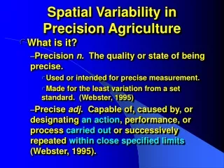
Agronomic Spatial Variability and Resolution What is it? How do we describe it? What does it imply for precision management?
Agronomic Variability • Fundamental assumption of precision farming • Agronomic factors vary spatially within a field • If these factors can be measured then crop yield and/or net economic returns can be optimize
Soils Classification Texture Organic matter Water holding capacity Topography Slope Aspect Fertility pH Nitrogen Phosphorus Potassium Other nutrients Plant available water Crop Cultivar Agronomic Variables
Temperature Rainfall Weeds Species Population Insects Species Feeding patterns Tillage Practices Soil Compaction Diseases Macro and micro environment Crop Stand Method and Uniformity of Application Fertilizers Crop protectants Agronomic Variables
What is variability • Variability - difference in the magnitude of measurements of a variable • Values can change randomly because of error in the sensor • Systematic error or bias • Values can change because of changes in the underlying factor • As time changes (Temporal) • As location changes (Spatial)
Why statistically describe measurements? • Raw data sets are too large to understand or interpret • Statistics provide a means of summarizing data and can be readily interpreted for making management decisions • Statistics can define relationships among variables
Statistical Analyses Commonly Used In Precision Agriculture • Descriptive Statistics • Measures of Central Tendency • Mean • Median • Measures of Dispersion • Range • Standard Deviation • Coefficient of Variation • Normal Distributions • Regression • Geostatistics - Semivariance Analysis
Measures of Central Tendency • When a factor, such as crop yield, is measured at different locations within a field, values may vary greatly • This variation can appear to be random • The set of these measurements is a population • A value exists that is the central or usual value of the population
Measures of Central Tendency • This is important because dimensions representing Biological Material are generally reported as single “expected”values.
Mean or Average Value • Most common measure of central tendency • Definition:For n measurements X1,X2,X3,…,Xn n å X + + + i X X . . . X = = = 1 2 1 n i X n n
Mean or Average • The mean or average value is useful if the measured value is normally distributed (Bell Curve) • Most biological processes are normally distributed • Spatially distributed measurements are often not normally distributed • To calculated the mean in Excel= Average (Col Row:Col Row)
Definition of (Col Row : Col Row) • Column letter of the upper left cell of an array of data • Row number of the upper left cell of an array of data • Column letter of the lower right cell of an array of data • Row number of the lower right cell of an array of data • The “:” instructs Excel to include all data between the two corner cells (Col Row:Col Row)
The Median Value • For skewed distributions, is the better predictor of the expected or central value • Calculated by ranking the values from high to low • For an odd number of measurements, the median is middle value • For an even number of measurements, the median is average of the two middle values • In Excel, the median is calculated using the following formula:= Median (Col Row : Col Row)
Normal vs. Skewed Distribution Mean Median Normal Normal Skewed Skewed Skewed Normal
Normality • Biological materials physical measurements are generally normally distributed about the mean. There are several test of normality which will be discussed in your statistics courses. However, three “quick and dirty” tests can be accessed easily from Excel • The first is simply comparing the mean and median values. If the values are nearly the same the measurement is likely distributed normally. • Excel has function calls to calculate Skewness and Kutrosis. These statistics can be used to test for nomality
Normality • Kurtosis measures deviation from the mean. A value of ‘0’ indicates that there is no deviation from a normal distribution. A positive value indicates that more values are clustered near the mean or far from it. A negative value means a “flat” top of the curve. • = Kurt (Col Row : Col Row)
Normality • Skewness is a measure of the tail of the distribution. A positive value indicates that there is an asymetrical tail of the distribution and that it is positive. A negative value indicates that there is a negative tail to the distribution. • =Skew (Col Row : Col Row)
Measures of Dispersion • Measures of dispersion describe the distribution of the set of measurements
Maximum and Minimum Values • The maximum value is the highest value in the data set • In Excel the maximum value is calculated by: = Max(Col Row:Col Row) • The minimum value is the lowest value in the data set and is calculated by:= Min(Col Row:Col Row)
Range of the Sample Set • Difference between the maximum and minimum values of the measurement • Calculated in Excel by the following formula:= Max (Col Row:Col Row) - Min (Col Row:Col Row)
Standard Deviation • The standard deviation of a normally distributed sample set is 1/2 of the “range” or ≈68 %values for the population n å 2 - ( X X ) i = = 1 i s - n 1
- £ £ + X 1 . 96 s Z X 1 . 96 s Standard Deviation • For a normal distribution (Bell Curve) ≈ 95% of the samples from a population will lie in the interval Where: X is the mean(average) value Z is a value (measurement) s is the standard deviation • The standard deviation is calculated in Excel using the following formula:= Stdev (Col Row : Col Row)
Coefficient of Variation • The magnitudes of the differences between large values and their means tend to be large. The differences between small values and their means tend to be small. • Consequently, a high yielding field is likely to have a higher standard deviation than a low yielding field, even if the variability is lower in the high yield field or the same as the lower yielding field.
Coefficient of Variation • Thus, variation about two means of different magnitudes cannot easily be compared. • Comparisons can be made by calculating the relative variation, or the normalized standard deviation. • This measurement is called the Coefficient of Variation.
Coefficient of Variation • The Coefficient of Variation or C.V. is calculated by dividing the standard deviation of the data set by its mean. Often that value is multiplied by 100 and the C.V. is expressed as a percentage. • Experience with similar data sets is required to determine if the C.V. is unusually large.
Mean, Standard Deviation and Coefficient of Variation Population = Y Mean Plant Spacing Std. Dev. = s CV Population = ½ Y Mean Plant Spacing Std. Dev. CV
Correlation • One objective of Biosystems engineering and Agronomy is to alter the level of one variable (e.g. soil nitrate) to change the response of another variable (e.g. grain yield). • There are other confounding factors affecting grain yield, such as soil pH, which cannot always be accounted for.
Correlation • The engineer still needs to determine the degree to which the two variables vary together. • The correlation coefficientor r is that measure. • The correlation coefficient, r, lies between -1 and 1. Positive values indicate that X and Y tend to increase or decrease together.
Correlation • Values of rnear 0 indicate that there is little or no relationship between the two variables. • The coefficient of determination or r2 is important in precision farming because, when the samples are collected by location in the field, it indicates the percentage of the variability in the dependent variable (e.g. yield) explained by the independent variable (e.g. N fertilizer).
Correlation • For example, if the r2 of soil N and grain yield is 90% then 90% of the variability across the field can be explained by soil nitrate. Spatially varying the N fertilizer rate based on the nitrate level in the soil should have a large effect on grain yield. • In Excel, correlation r is calculate by the following:= Correl (Col Row : Col Row, Col Row: Col Row) To calculate r2, simply square the value of r.
Regression • Excel has the capability of fitting mathematical models (linear and non-linear curves) to data which relate dependent to independent variables. Regression (curve fitting) can be performed using the Charting GUI in Excel. You can also directly calculate the slope and intercept for a linear model using the commands
Regression • = Intercept (Col Row : Col Row)and • = Slope (Col Row : Col Row) • Regression R2 is a measure in decimal percent of how well the model fits the data. For linear regression, the regression R2 can be directly calculated be squareing the correlation coefficient
High Resolution Variability Study – 1 ft x 1ft Experiments