Download
1 / 23
230 likes | 406 Views
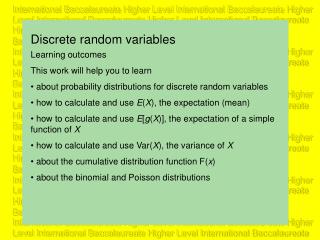
Section 7.1.1 Discrete and Continuous Random Variables. AP Statistics. Random Variables. A random variable is a variable whose value is a numerical outcome of a random phenomenon. For example: Flip three coins and let X represent the number of heads. X is a random variable.

E N D
Section 7.1.1Discrete and Continuous Random Variables AP Statistics
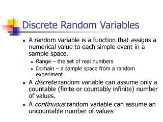
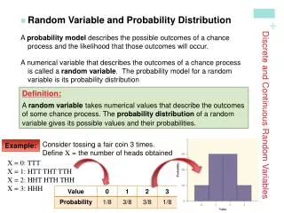
Random Variables • A random variable is a variable whose value is a numerical outcome of a random phenomenon. • For example: Flip three coins and let X represent the number of heads. X is a random variable. • We usually use capital letters to denotes random variables. • The sample space S lists the possible values of the random variable X. • We can use a table to show the probability distribution of a discrete random variable. AP Statistics, Section 7.1, Part 1
Discrete Probability Distribution Table AP Statistics, Section 7.1, Part 1
Discrete Random Variables • A discrete random variable X has a countable number of possible values. The probability distribution of X lists the values and their probabilities. X: x1 x2 x3 … xk P(X): p1 p2 p3 … pk 1. 0 ≤ pi ≤ 1 2. p1 + p2 + p3 +… + pk = 1. AP Statistics, Section 7.1, Part 1
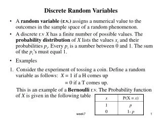
Probability Distribution Table: Number of Heads Flipping 4 Coins AP Statistics, Section 7.1, Part 1
Probabilities: • X: 0 1 2 3 4 • P(X): 1/16 1/4 3/8 1/4 1/16 .0625 .25 .375 .25 .0625 • Histogram AP Statistics, Section 7.1, Part 1
Questions. • Using the previous probability distribution for the discrete random variable X that counts for the number of heads in four tosses of a coin. What are the probabilities for the following? • P(X = 2) • P(X ≥ 2) • P(X ≥ 1) .375 .375 + .25 + .0625 = .6875 1-.0625 = .9375 AP Statistics, Section 7.1, Part 1
What is the average number of heads? AP Statistics, Section 7.1, Part 1
Continuous Random Varibles • Suppose we were to randomly generate a decimal number between 0 and 1. There are infinitely many possible outcomes so we clearly do not have a discrete random variable. • How could we make a probability distribution? • We will use a density curve, and the probability that an event occurs will be in terms of area. AP Statistics, Section 7.1, Part 1
Definition: • A continuous random variable X takes all values in an interval of numbers. • The probability distribution of X is described by a density curve. The Probability of any event is the area under the density curve and above the values of X that make up the event. • All continuous random distributions assign probability 0 to every individual outcome. AP Statistics, Section 7.1, Part 1
Distribution of Continuous Random Variable AP Statistics, Section 7.1, Part 1
Example of a non-uniform probability distribution of a continuous random variable. AP Statistics, Section 7.1, Part 1
Problem • Let X be the amount of time (in minutes) that a particular San Francisco commuter must wait for a BART train. Suppose that the density curve is a uniform distribution. • Draw the density curve. • What is the probability that the wait is between 12 and 20 minutes? AP Statistics, Section 7.1, Part 1
Density Curve. AP Statistics, Section 7.1, Part 1
Probability shaded. P(12≤ X ≤ 20) = 0.5 · 8 = .40 AP Statistics, Section 7.1, Part 1
Normal Curves • We’ve studied a density curve for a continuous random variable before with the normal distribution. • Recall: N(μ, σ) is the normal curve with mean μ and standard deviation σ. • If X is a random variable with distribution N(μ, σ), then is N(0, 1) AP Statistics, Section 7.1, Part 1
Example • Students are reluctant to report cheating by other students. A sample survey puts this question to an SRS of 400 undergraduates: “You witness two students cheating on a quiz. Do you go to the professor and report the cheating?” • Suppose that if we could ask all undergraduates, 12% would answer “Yes.” The proportion p = 0.12 would be a parameter for the population of all undergraduates. AP Statistics, Section 7.1, Part 1
Example continued • Students are reluctant to report cheating by other students. A sample survey puts this question to an SRS of 400 undergraduates: “You witness two students cheating on a quiz. Do you go to the professor and report the cheating?” • What is the probability that the survey results differs from the truth about the population by more than 2 percentage points? • Because p = 0.12, the survey misses by more than 2 percentage points if AP Statistics, Section 7.1, Part 1
Example continued Calculations About 21% of sample results will be off by more than two percentage points. AP Statistics, Section 7.1, Part 1
Summary • A discrete random variable X has a countable number of possible values. • The probability distribution of X lists the values and their probabilities. • A continuous random variable X takes all values in an interval of numbers. • The probability distribution of X is described by a density curve. The Probability of any event is the area under the density curve and above the values of X that make up the event. AP Statistics, Section 7.1, Part 1
Summary • When you work problems, first identify the variable of interest. • X = number of _____ for discrete random variables. • X = amount of _____ for continuous random variables. AP Statistics, Section 7.1, Part 1