Download
1 / 11
330 likes | 1.81k Views
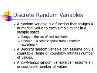
Discrete Random Variables. A random variable (r.v.) assigns a numerical value to the outcomes in the sample space of a random phenomenon.

E N D
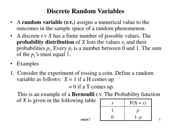
Discrete Random Variables • A random variable (r.v.) assigns a numerical value to the outcomes in the sample space of a random phenomenon. • A discrete r.v X has a finite number of possible values. The probability distribution of X lists the values xi and their probabilities pi. Every pi is a number between 0 and 1. The sum of the pi’s must equal 1. • Examples 1. Consider the experiment of tossing a coin. Define a random variable as follows: X = 1 if a H comes up = 0 if a T comes up. This is an example of a Bernoulli r.v. The Probability function of X is given in the following table week7
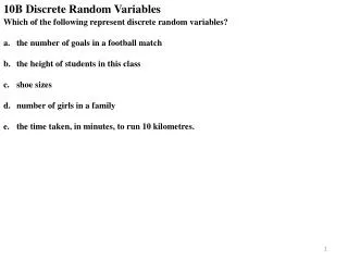
Let X be a r.v counting the number of girls in a family with 3 children. The probability function of X is given in the following table. • Toss a coin 4 times. Let X be the number of H’s. Find the probability function of X. Draw a probability histogram. • Toss a coin until the 1st H. Let X be the number of T’s before the 1st H. Find the probability function of X. week7
Continuous random variables • A continuous r. v. X takes all values in an interval of numbers. • The probability distribution of X is described by a density curve. • The total area under a density curve is 1. • The probability of any event is the area under the density curve and above the value of X that make up the event. • Example The density function of a continuous r. v. X is given in the graph below. Find i) P(X < 7) ii) P(6 < X < 8) iii) P(X = 7) iv) P(5.5 < X < 7 or 8 < X < 9) week7
Normal distributions The density curves that are most familiar to us are the normal curves. week7
Mean (expected value) of a discrete r. v. • The mean of a r. v. X is denoted by μx and can be found using the following formula: • Examples: 1. The mean of the Bernoulli r.v defined in example 1 above is : μx= 0·(1-p) + 1·p = p 2. The mean number of girls in a family with 3 children is 1.5. • Exercise: Find the mean of X in example 3 above. • Exercise: Read Example 4.20 on p291 in IPS. week7
Example – Discrete Uniform r.v • Roll a six-sided die. Define a r. v. X to be the number shown on the die. That is, X = 1 if die lands on 1, X = 2 if die lands on 2, etc. The probability distribution of X is given in the table below: The mean of X is μX = 1·(1/6) + 2·(1/6) + 3·(1/6) + 4·(1/6) +5·(1/6) + 6·(1/6) = 21/6 = 3.5 . week7
Law of large numbers • If independent observations are drawn from a population with a finite mean , the population mean can be estimated with a specified degree of accuracy by the sample mean , using sufficiently large sample. week7
Rules for Mean of r.v • For any two r.v’s X and Y and constants a and b, 1. μx + a = μx + a . 2. μb·x = b·μx . 3. μb·x + a = b·μx + a . 4. μX + Y = μX + μY. • Example: The price X of Nike sports shoes is a random variable with mean μx = 200$. Before the holidays Nike company had a promotion: “ Pay 10$ less for each item and get 20% discount from the original price”. • What is the mean price during the promotion. • Suppose in addition that during the promotion the mean price for Nike socks is μY = 20$. What is the expected value of your expenses if you are to buy one pair of shoes and one pair of socks ? week7
The variance of a r. v. • The variance of a r. v. is an average of the squared deviations from the mean, (X – μx)2 . • The Variance of a discrete r. v. is • The standard deviationσX of a r. v. is the square root of its variance. • Examples: • The variance of a Bernoulli r.v is σ2x = p – p2 = p(1- p) 2. The variance of the Uniform example above is σ2x = (91/6) – (3.5)2 = 2.9167 week7
Rules for variances • If X is a r. v. and a and b are constants, then 1. 2. 3. 4. If X and Y are independent r. v’s then, week7
Two random variables X and Y are independent if knowing that any event involving X alone did or did not occur tells us nothing about the occurrence of any event involving Y alone. • Example: Consider again the Nike example above. If the stdev. of X is σx = 10$ and the stdev. of Y is σY = 8$. • What is the stdev. of the shoes price during the promotion? (8). • What is the stdev. of your expenses if you were to buy one pair of shoes and one pair of socks ? (12.806). • Example 4.34 on page 283 in IPS. week7