Download
1 / 51
550 likes | 842 Views
Introduction To Resonant Circuits. University of Tennessee, Knoxville ECE Department. wlg. Resonance In Electric Circuits. Any passive electric circuit will resonate if it has an inductor and capacitor. . . Resonance is characterized by the input voltage and current

E N D
Introduction To Resonant Circuits University of Tennessee, Knoxville ECE Department wlg
Resonance In Electric Circuits Any passive electric circuit will resonate if it has an inductor and capacitor. Resonance is characterized by the input voltage and current being in phase. The driving point impedance (or admittance) is completely real when this condition exists. In this presentation we will consider (a) series resonance, and (b) parallel resonance.
Series Resonance Consider the series RLC circuit shown below. V = VM 0 R L + C V I _ The input impedance is given by: The magnitude of the circuit current is;
Series Resonance Resonance occurs when, At resonance we designate w as wo and write; This is an important equation to remember. It applies to both series And parallel resonant circuits.
Series Resonance The magnitude of the current response for the series resonance circuit is as shown below. |I| Half power point w1 wo w2 w Bandwidth: BW = wBW = w2 – w1
Series Resonance The peak power delivered to the circuit is; . The so-called half-power is given when We find the frequencies, w1 and w2, at which this half-power occurs by using;
Series Resonance After some insightful algebra one will find two frequencies at which the previous equation is satisfied, they are: and The two half-power frequencies are related to the resonant frequency by
Series Resonance The bandwidth of the series resonant circuit is given by; We define the Q (quality factor) of the circuit as; Using Q, we can write the bandwidth as; These are all important relationships.
Series Resonance An Observation: If Q > 10, one can safely use the approximation; These are useful approximations.
Series Resonance An Observation: By using Q = woL/R in the equations for w1and w2 we have; and
Series Resonance In order to get some feel for how the numerical value of Q influences the resonant and also get a better appreciation of the s-plane, we consider the following example. It is easy to show the following for the series RLC circuit. In the following example, three cases for the about transfer function will be considered. We will keep wo the same for all three cases. The numerator gain,k, will (a) first be set k to 2 for the three cases, then (b) the value of k will be set so that each response is 1 at resonance.
Series Resonance An Example Illustrating Resonance: The 3 transfer functions considered are: Case 1: Case 2: Case 3:
Series Resonance An Example Illustrating Resonance: The poles for the three cases are given below. Case 1: Case 2: Case 3:
Series Resonance Comments: Observe the denominator of the CE equation. Compare to actual characteristic equation forCase 1: rad/sec rad/sec
Series Resonance Poles and Zeros In the s-plane: jw axis ( 3) (2) (1) x 20 x x s-plane axis 0 -1 -5 -2.5 0 Note the location of the poles for the three cases. Also note there is a zero at the origin. x x x -20 ( 3) (2) (1)
Series Resonance Comments: The frequency response starts at the origin in the s-plane. At the origin the transfer function is zero because there is a zero at the origin. As you get closer and closer to the complex pole, which has a j parts in the neighborhood of 20, the response starts to increase. The response continues to increase until we reach w = 20. From there on the response decreases. We should be able to reason through why the response has the above characteristics, using a graphical approach.
Series Resonance Matlab Program For The Study: % name of program is freqtest.m % written for 202 S2002, wlg %CASE ONE DATA: K = 2; num1 = [K 0]; den1 = [1 2 400]; num2 = [K 0]; den2 = [1 5 400]; num3 = [K 0]; den3 = [1 10 400]; w = .1:.1:60; grid H1 = bode(num1,den1,w); magH1=abs(H1); H2 = bode(num2,den2,w); magH2=abs(H2); H3 = bode(num3,den3,w); magH3=abs(H3); plot(w,magH1, w, magH2, w,magH3) grid xlabel('w(rad/sec)') ylabel('Amplitude') gtext('Q = 10, 4, 2')
Series Resonance Program Output
Series Resonance Comments: cont. From earlier work: With Q = 10, this gives; w1= 19.51 rad/sec, w2 = 20.51 rad/sec Compare this to the approximation: w1 = w0 – BW = 20 – 1 = 19 rad/sec, w2 = 21 rad/sec So basically we can find all the series resonant parameters if we are given the numerical form of the CE of the transfer function.
Series Resonance Next Case: Normalize all responses to 1 at wo
Series Resonance Three dB Calculations: Now we use the analytical expressions to calculate w1 and w2. We will then compare these values to what we find from the Matlab simulation. Using the following equations with Q = 2, we find, w1 = 15.62 rad/sec w2 = 21.62 rad/sec
Series Resonance Checking w1 and w2 (cut-outs from the simulation) 25.3000 0.7254 25.4000 0.7195 25.5000 0.7137 25.6000 0.7080 25.7000 0.7023 25.8000 0.6967 25.9000 0.6912 15.3000 0.6779 15.4000 0.6871 15.5000 0.6964 15.6000 0.7057 15.7000 0.7150 15.8000 0.7244 w2 w1 This verifies the previous calculations. Now we shall look at Parallel Resonance.
Parallel Resonance Background Consider the circuits shown below: V I R L C L R V C I
Series Resonance Duality We notice the above equations are the same provided: If we make the inner-change, then one equation becomes the same as the other. For such case, we say the one circuit is the dual of the other. If we make the inner-change, then one equation becomes the same as the other. For such case, we say the one circuit is the dual of the other.
Parallel Resonance Background What this means is that for all the equations we have derived for the parallel resonant circuit, we can use for the series resonant circuit provided we make the substitutions: What this means is that for all the equations we have derived for the parallel resonant circuit, we can use for the series resonant circuit provided we make the substitutions: What this means is that for all the equations we have derived for the parallel resonant circuit, we can use for the series resonant circuit provided we make the substitutions:
Parallel Resonance Parallel Resonance Series Resonance
Resonance Example 1: Determine the resonant frequency for the circuit below. At resonance, the phase angle of Z must be equal to zero.
Resonance Analysis For zero phase; This gives; or
Parallel Resonance Example 2: A parallel RLC resonant circuit has a resonant frequency admittance of 2x10⁻² S(mohs). The Q of the circuit is 50, and the resonant frequency is 10,000 rad/sec. Calculate the values of R, L, and C. Find the half-power frequencies and the bandwidth. A parallel RLC resonant circuit has a resonant frequency admittance of 2x10⁻² S(mohs). The Q of the circuit is 50, and the resonant frequency is 10,000 rad/sec. Calculate the values of R, L, and C. Find the half-power frequencies and the bandwidth. A series RLC resonant circuit has a resonant frequency admittance of 2x10⁻² S(mohs). The Q of the circuit is 50, and the resonant frequency is 10,000 rad/sec. Calculate the values of R, L, and C. Find the half-power frequencies and the bandwidth. First, R = 1/G = 1/(0.02) = 50 ohms. , we solve for L, knowing Q, R, and wo to Second, from find L = 0.25 H. Third, we can use
Parallel Resonance Example 2: (continued) Fourth: We can use and Fifth: Use the approximations; w1 = wo - 0.5wBW = 10,000 – 100 = 9,900 rad/sec w2 = wo - 0.5wBW = 10,000 + 100 = 10,100 rad/sec
Extension of Series Resonance Peak Voltages and Resonance: VR VL _ _ + + L R + + VC C VS I _ _ We know the following: When w = wo = , VS and I are in phase, the driving point impedance is purely real and equal to R. A plot of |I| shows that it is maximum at w = wo. We know the standard equations for series resonance applies: Q, wBW, etc.
Extension of Series Resonance Reflection: A question that arises is what is the nature of VR, VL, and VC? A little reflection shows that VR is a peak value at wo. But we are not sure about the other two voltages. We know that at resonance they are equal and they have a magnitude of QxVS. Irwin shows that the frequency at which the voltage across the capacitor is a maximum is given by; Irwin shows that the frequency at which the voltage across the capacitor is a maximum is given by; Irwin shows that the frequency at which the voltage across the capacitor is a maximum is given by; The above being true, we might ask, what is the frequency at which the voltage across the inductor is a maximum? We answer this question by simulation
Extension of Series Resonance Series RLC Transfer Functions: The following transfer functions apply to the series RLC circuit.
Extension of Series Resonance Parameter Selection: We select values of R, L. and C for this first case so that Q = 2 and wo = 2000 rad/sec. Appropriate values are; R = 50 ohms, L = .05 H, C = 5F. The transfer functions become as follows:
Extension of Series Resonance Matlab Simulation: grid HC = bode(numC,denC,w); magHC = abs(HC); HL = bode(numL,denL,w); magHL = abs(HL); HR = bode(numR,denR,w); magHR = abs(HR); plot(w,magHC,'k-', w, magHL,'k--', w, magHR, 'k:') grid xlabel('w(rad/sec)') ylabel('Amplitude') title(' Rsesponse for RLC series circuit, Q =2') gtext('VC') gtext('VL') gtext(' VR') % program is freqcompare.m % written for 202 S2002, wlg numC = 4e+6; denC = [1 1000 4e+6]; numL = [1 0 0]; denL = [1 1000 4e+6]; numR = [1000 0]; denR = [1 1000 4e+6]; w = 200:1:4000; grid HC = bode(numC,denC,w); magHC = abs(HC);
Exnsion of Series Resonance Simulation Results Q = 2
Exnsion of Series Resonance Analysis of the problem: Given the previous circuit. Find Q, w0, wmax, |Vc| at wo, and |Vc| at wmax VR VL _ _ + + R=50 L=5 mH + + VC C=5 F VS I _ _ Solution:
Exnsion of Series Resonance Problem Solution: Now check the computer printout.
Exnsion of Series Resonance Problem Solution (Simulation): 1.0e+003 * 1.8600000 0.002065141 1.8620000 0.002065292 1.8640000 0.002065411 1.8660000 0.002065501 1.8680000 0.002065560 1.8700000 0.002065588 1.8720000 0.002065585 1.8740000 0.002065552 1.8760000 0.002065487 1.8780000 0.002065392 1.8800000 0.002065265 1.8820000 0.002065107 1.8840000 0.002064917 Maximum
Extension of Series Resonance Simulation Results: Q=10
Exnsion of Series Resonance Observations From The Study: The voltage across the capacitor and inductor for a series RLC circuit is not at peak values at resonance for small Q (Q <3). Even for Q<3, the voltages across the capacitor and inductor are equal at resonance and their values will be QxVS. For Q>10, the voltages across the capacitors are for all practical purposes at their peak values and will be QxVS. Regardless of the value of Q, the voltage across the resistor reaches its peak value at w = wo. For high Q, the equations discussed for series RLC resonance can be applied to any voltage in the RLC circuit. For Q<3, this is not true.
Extension of Resonant Circuits Given the following circuit: + R + C V I L _ _ We want to find the frequency, wr, at which the transfer function for V/I will resonate. The transfer function will exhibit resonance when the phase angle between V and I are zero.
Extension of Resonant Circuits The desired transfer functions is; This equation can be simplified to; With s jw
Extension of Resonant Circuits Resonant Condition: For the previous transfer function to be at a resonant point, the phase angle of the numerator must be equal to the phase angle of the denominator. or, . , Therefore;
Extension of Resonant Circuits Resonant Condition Analysis: Canceling the w’s in the numerator and cross multiplying gives, This gives, Notice that if the ratio of R/L is small compared to 1/LC, we have
Extension of Resonant Circuits Resonant Condition Analysis: What is the significance of wr and wo in the previous two equations? Clearly wr is a lower frequency of the two. To answer this question, consider the following example. Given the following circuit with the indicated parameters. Write a Matlab program that will determine the frequency response of the transfer function of the voltage to the current as indicated. + R + C V I L _ _
Extension of Resonant Circuits Resonant Condition Analysis: Matlab Simulation: We consider two cases: Case 1: Case 2: R = 3 ohms C = 6.25x10⁻⁵ F L = 0.01 H R = 1 ohms C = 6.25x10⁻⁵ F L = 0.01 H wr= 2646 rad/sec wr= 3873 rad/sec For both cases, wo = 4000 rad/sec
Extension of Resonant Circuits Resonant Condition Analysis: Matlab Simulation: The transfer functions to be simulated are given below. Case 1: Case 2:
Extension of Resonant Circuits 2646 rad/sec
Extension of Resonant Circuits What can be learned from this example? wr does not seem to have much meaning in this problem. What is wr if R = 3.99 ohms? Just because a circuit is operated at the resonant frequency does not mean it will have a peak in the response at the frequency. For circuits that are fairly complicated and can resonant, It is probably easier to use a simulation program similar to Matlab to find out what is going on in the circuit.