Download
1 / 42
420 likes | 427 Views
Self-optimizing control: Simple implementation of optimal operation. Sigurd Skogestad Department of Chemical Engineering Norwegian University of Science and Tecnology (NTNU) Trondheim, Norway Benelux Control Meeting, March 2008

E N D
Self-optimizing control:Simple implementation ofoptimal operation Sigurd Skogestad Department of Chemical Engineering Norwegian University of Science and Tecnology (NTNU) Trondheim, Norway Benelux Control Meeting, March 2008 PART 2: Effective Implementation of optimal operation using Off-Line Computations
Outline • Implementation of optimal operation • Paradigm 1: On-line optimizing control • Paradigm 2: "Self-optimizing" control schemes • Precomputed (off-line) solution • Control of optimal measurement combinations • Nullspace method • Exact local method • Link to optimal control / Explicit MPC • Current research issues
Optimal operation • A typical dynamic optimization problem • Implementation: “Open-loop” solutions not robust to disturbances or model errors • Want to introduce feedback
Implementation of optimal operation • Paradigm 1:On-line optimizing control where measurements are used to update model and states • Paradigm 2: “Self-optimizing” control scheme found by exploiting properties of the solution in control structure design • Usually feedback solutions • Use off-line analysis/optimization to find “properties of the solution” • “self-optimizing ” = “inherent optimal operation”
Implementation: Paradigm 1 • Paradigm 1: Online optimizing control • Measurements are primarily used to update the model • The optimization problem is resolved online to compute new inputs. • Example: Conventional MPC • This is the “obvious” approach (for someone who does not know control)
Example paradigm 1: Marathon runner • Even getting a reasonable model requires > 10 PhD’s … and the model has to be fitted to each individual…. • Clearly impractical!
Implementation: Paradigm 2 • Paradigm 2: Precomputed solutions based on off-line optimization • Find properties of the solution suited for simple and robust on-line implementation • Examples • Marathon runner • Hierarchical decomposition • Optimal control • Explicit MPC
Example paradigm 2: Marathon runner select one measurement c = heart rate • Simple and robust implementation • Disturbances are indirectly handled by keeping a constant heart rate • May have infrequent adjustment of setpoint (heart rate)
Example paradigm 2: Optimal operation of chemical plant • Hierarchial decomposition based on time scale separation Self-optimizing control: Acceptable operation (=acceptable loss) achieved using constant set points (cs) for the controlled variables c cs • No or infrequent online optimization. • Controlled variables c are found based on off-line analysis.
Example paradigm 2: Feedback implementation of optimal control (LQ) • Optimal solution to infinite time dynamic optimization problem • Originally formulated as a “open-loop” optimization problem (no feedback) • “By chance” the optimal u can be generated by simple state feedback u = KLQ x • KLQ is obtained off-line by solving Riccatti equations • Explicit MPC: Extension using different KLQ in each constraint region • Summary: Two paradigms MPC • Conventional MPC: On-line optimization • Explicit MPC: Off-line calculation of KLQ for each region (must determine regions online)
Example paradigm 2: Explicit MPC MPC: Model predictive control Note: Many regions because of future constraints A. Bemporad, M. Morari, V. Dua, E.N. Pistikopoulos, ”The Explicit Linear Quadratic Regulator for Constrained Systems”, Automatica, vol. 38, no. 1, pp. 3-20 (2002).
Issues Paradigm 2: Precomputed on-line solutions based on off-line optimization Issues (expected research results for specific application): • Find structure of optimal solution for specific problems • Typically, identify regions where different set of constraints are active • Find optimal values (or trajectories) for unconstrained variables • Find analytical or precomputed solutions suitable for on-line implementation • Find good “self-optimizing” variables c to control in each region • Find good variable combinations to control • Determine a switching policy between different regions
Unconstrained degrees of freedom: How find “self-optimizing” variable combinations in a systematic manner? • The ideal “self-optimizing” variable is the gradient (first-order optimality condition (ref: Bonvin and coworkers)): • Optimal setpoint = 0 • BUT: Gradient can not be measured in practice • Possible approach: Estimate gradient Ju based on measurements y • Here alternative approach: Find optimal linear measurement combination which when kept constant ( § n) minimize the effect of d on loss. Loss = J(u,d) – J(uopt,d); where u is input for c = constant § n • Candidate measurements (y): Include also inputs u
Unconstrained degrees of freedom: B. Optimal measurement combination H
Unconstrained degrees of freedom: B. Optimal measurement combination B1. Nullspace method for n = 0 (Alstad and Skogestad, 2007) Basis: Want optimal value of c to be independent of disturbances • Find optimal solution as a function of d: uopt(d), yopt(d) • Linearize this relationship: yopt= F d • Want: • To achieve this for all values of d: • To find a F that satisfies HF=0 we must require • Optimal when we disregard implementation error (n) Amazingly simple! Sigurd is told how easy it is to find H V. Alstad and S. Skogestad, ``Null Space Method for Selecting Optimal Measurement Combinations as Controlled Variables'', Ind.Eng.Chem.Res, 46 (3), 846-853 (2007).
Unconstrained degrees of freedom: B. Optimal measurement combination B2. Combined disturbances and implementation errors (“exact local method”) Loss L = J(u,d) – Jopt(d). Keep c = Hy constant , where y = Gyu + Gydd + ny Theorem 1. Worst-case loss for given H(Halvorsen et al, 2003): Applies to any H (selection/combination) Optimization problem for optimal combination: • I.J. Halvorsen, S. Skogestad, J.C. Morud and V. Alstad, ``Optimal selection of controlled variables'', Ind. Eng. Chem. Res., 42 (14), 3273-3284 (2003).
Unconstrained degrees of freedom: B. Optimal measurement combination B2. Exact local method for combined disturbances and implementation errors. Theorem 2. Explicit formula for optimal H. (Alstad et al, 2008): • F – optimal sensitivity matrix = dyopt/dd Theorem 3. (Kariwala et al, 2008). V. Alstad, S. Skogestad and E.S. Hori, ``Optimal measurement combinations as controlled variables'', Journal of Process Control, 18, in press (2008). V. Kariwala, Y. Cao, S. jarardhanan, “Local self-optimizing control with average loss minimization”, Ind.Eng.Chem.Res., in press (2008)
Toy Example: Single measurements Constant input, c = y4 = u Want loss < 0.1: Consider variable combinations
B1. Nullspace method (no noise) • Loss caused by measurement error only • Recall rank single measurements: 3 > 2 > 4 > 1
B2. Exact local method, 2 measurements Combined loss for disturbances and measurement errors
Example: CO2 refrigeration cycle Unconstrained DOF (u) Control what? c=? pH
CO2 refrigeration cycle Step 1. One (remaining) degree of freedom (u=z) Step 2. Objective function. J = Ws (compressor work) Step 3. Optimize operation for disturbances (d1=TC, d2=TH, d3=UA) • Optimum always unconstrained Step 4. Implementation of optimal operation • No good single measurements (all give large losses): • ph, Th, z, … • Nullspace method: Need to combine nu+nd=1+3=4 measurements to have zero disturbance loss • Simpler: Try combining two measurements. Exact local method: • c = h1 ph + h2 Th = ph + k Th; k = -8.53 bar/K • Nonlinear evaluation of loss: OK!
Refrigeration cycle: Proposed control structure Control c= “temperature-corrected high pressure”
Summary: Procedure selection controlled variables • Define economics and operational constraints • Identify degrees of freedom and important disturbances • Optimize for various disturbances • Identify active constraints regions (off-line calculations) For each active constraint region do step 5-6: 5. Identify “self-optimizing” controlled variables for remaining degrees of freedom 6. Identify switching policies between regions
Example switching policies – 10 km • ”Startup”: Given speed or follow ”hare” • When heart beat > max or pain > max: Switch to slower speed • When close to finish: Switch to max. power Another example: Regions for LNG plant (see Chapter 7 in thesis by J.B.Jensen, 2008)
Current research 1 (Sridharakumar Narasimhan and Henrik Manum):Conditions for switching between regions of active constraints Idea: • Within each region it is optimal to • Control active constraints at ca = c,a, constraint • Control self-optimizing variables at cso = c,so, optimal • Define in each region i: • Keep track of ci (active constraints and “self-optimizing” variables) in all regions i • Switch to region i when element in ci changes sign • Research issue: can we get lost?
Current research 2 (Håkon Dahl-Olsen):Extension to dynamic systems • Basis. From dynamic optimization: • Hamiltonian should be minimized along the trajectory • Generalize steady-state local methods: • Generalize maximum gain rule • Generalize nullspace method (n=0) • Generalize “exact local method”
Current research 3 (Sridharakumar Narasimhan and Johannes Jäschke):Extension of noise-free case (nullspace method) to nonlinear systems • Idea: The ideal self-optimizing variable is the gradient • Optimal setpoint = 0 • Certain problems (e.g. polynomial) • Find analytic expression for Ju in terms of u and d • Derive Ju as a function of measurements y (eliminate disturbances d)
Current research 4 (Henrik Manum and Sridharakumar Narasimhan):Self-optimizing control and Explicit MPC • Our results on optimal measurement combination (keep c = Hy constant) • Nullspace method for n=0 (Alstad and Skogestad, 2007) • Explicit expression (“exact local method”) for n≠0 (Alstad et al., 2008) • Observation 1: Both result are exact for quadratic optimization problems • Observation 2: MPC can be written as a quadratic optimization problem and optimal solution is to keep c = u – Kx constant. • Must be some link!
Quadratic optimization problems • Noise-free case (n=0) • Reformulation of nullspace method of Alstad and Skogestad (2007) • Can add linear constraints (c=Hy) to quadratic problem with no loss • Need ny ≥ nu + nd. H is unique if ny = nu + nd (nym = nd) • H may be computed from nullspace method, • V. Alstad and S. Skogestad, ``Null Space Method for Selecting Optimal Measurement Combinations as Controlled Variables'', Ind. Eng. Chem. Res, 46 (3), 846-853 (2007).
Quadratic optimization problems • With noise / implementation error (n ≠ 0) • Reformulation of exact local method of Alstad et al. (2008) • Can add linear constraints (c=Hy) with minimum loss. • Have explicit expression for H from “exact local method” • V. Alstad, S. Skogestad and E.S. Hori, ``Optimal measurement combinations as controlled variables'', Journal of Process Control, 18, in press (2008).
Optimal control / Explicit MPC • Treat initial state x0 as disturbance d. Discrete time constrained MPC problem: • In each active constraint region this becomes an unconstrained quadratic optimization problem )Can use above results to find linear constraints • State feedback with no noise (LQ problem) Measurements: y = [u x] Linear constraints: c = H y = u – K x • nx = nd: No loss (solution unchanged) by keeping c = 0, so u = Kx optimal! • Can find optimal feedback K from “nullspace method”, • Same result as solving Riccatti equations • NEW INSIGHT EXPLICIT MPC: Use change in sign of c for neighboring regions to decide when to switch regions • H. Manum, S. Narasimhan and S. Skogestad, ``A new approach to explicit MPC using self-optimizing control”, ACC, Seattle, June 2008.
Explicit MPC. State feedback.Second-order system Phase plane trajectory time [s]
Optimal control / Explicit MPC • Output feedback (All states not measured). No noise • Option 1: State estimator • Option 2: Direct use of measurements for feedback “Measurements”: y = [u ym] Linear constraints: c = H y = u – K ym • No loss (solution unchanged) by keeping c = 0 (constant), so u = Kym is optimal,provided we have enough independent measurements: ny ≥ nu + nd ) nym ≥ nd • Can find optimal feedback K from “self-optimizing nullspace method” • Can also add previous measurements, but get some loss due to causality (cannot affect past outputs) H. Manum, S. Narasimhan and S. Skogestad, ``Explicit MPC with output feedback using self-optimizing control”, IFAC World Congress, Seoul, July 2008.
Explicit MPC. Output feedbackSecond-order system State feedback time [s]
Optimal control / Explicit MPC 2. Output feedback – Further extensions • Explicit expressions for certain fix-order optimal controllers • Example: Can find optimal multivariable PID controller by using as “measurements” • Current output (P) • Sum of outputs (I) • Change in output (D)
Optimal control / Explicit MPC 3. Further extension: Output feedback with noise • Option 1: State estimator • Option 2: Direct use of measurements for feedback “Measurements”: y = [u ym] Linear constraints: c = H y = u – K ym • Loss by using this feedback law (adding these constraints) is minimized by computing feedback K using “exact local method” H. Manum, S. Narasimhan and S. Skogestad, ``Explicit MPC with output feedback using self-optimizing control”, IFAC World Congress, Seoul, July 2008.
Conclusion • Simple control policies are always preferred in practice (if they exist and can be found) • Paradigm 2: Use off-line optimization and analysis to find simple near-optimal control policies suitable for on-line implementation • Current research: Several interesting extensions • Optimal region switching • Dynamic optimization • Explicit MPC • Acknowledgements • Sridharakumar Narasimhan • Henrik Manum • Håkon Dahl-Olsen • Vinay Kariwala