Download
1 / 12
120 likes | 125 Views
Creation of Bathymetric Surfaces Using High-Density Point Surveys. Mark Schmelter CEE 6440 GIS in Water Resource Engineering Fall 2007. Relevance to W.R. Engineering. New methods of data collection and analysis are constantly evolving e.g., multi-dimensional hydraulic models

E N D
Creation of Bathymetric Surfaces Using High-Density Point Surveys Mark Schmelter CEE 6440 GIS in Water Resource Engineering Fall 2007
Relevance to W.R. Engineering • New methods of data collection and analysis are constantly evolving • e.g., multi-dimensional hydraulic models • e.g., LiDAR, SoNAR • Hydraulics = f(bathymetry, planform) • Habitat models rely upon hydraulics • Geomorphic models rely upon hydraulics • Etc.
Objectives • Evaluate: • Differences between interpolation methods • Differences between interpolated surfaces resulting from differing point densities
Data and their Origins • Point data file from Trinity River Restoration Project (TRRP) • Collected using Airborne LiDAR Bathymetry (ALB) technology • Helicopter-mounted green and infra-red LiDAR • Horizontal precision = 2.5m • Vertical precision = 0.25m • Rated to water depth of 50m in ‘good’ conditions • Trinity data collected in December 2003 (6m max depth)
"Everything is related to everything else, but near things are more related than distant things" (Tobler 1970) • Inverse Distance Weighted • Fast, very simple algorithm, easy paramaterization • Ordinary Kriging • Not fast, complicated parameterization • Robust statistical method • Local Polynomial Interpolation • Fast, easy parameterization (idiot-proof?) • Complicated; fits polynomial eqns to data Tobler, W. R. (1970). "A computer model simulation of urban growth in the Detroit region." Economic Geography, 46(2), 234-240.
Full dataset 10% of full dataset 100% 85% 70% 55% 40% 25% 10%
Reminder of objectives 1 & 2 • See how surfaces vary between methods • See how surfaces vary with changing point densities
Metrics • RMSE • Mean residuals • Time to compute • Cross-validation: • Remove one point from the data, interpolate, then compare the interpolated value at the removed location to the removed value Red: Mean residual = -4.498; RMSE = 8.094 Black: Mean residual = 0.1142; RMSE = -2.817
RMSE Mean Residual Time to compute
In the end… • 12:12 versus 0:46 • Unless you need to have a standard deviation surface (e.g., to create a confidence interval on your surface), just use IDW or LPI • If you want to have a confidence interval on your surface, you must use kriging
Questions? Kriged map of 55% subset Standard deviation map of 55% subset