Download
1 / 19
190 likes | 347 Views
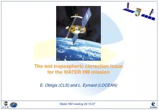
The wet tropospheric correction for coastal altimetry. L. Eymard. C. Desportes. T. Strub. E. Obligis. R. Scharroo. G. Wick. B. Khayatian. S. Brown. T. Haack. F. Mercier. OUTLINE What do we know about coastal water vapor and the distance and time scales over which it changes ?

E N D
The wet tropospheric correction for coastal altimetry L. Eymard C. Desportes T. Strub E. Obligis R. Scharroo G. Wick B. Khayatian S. Brown T. Haack F. Mercier
OUTLINE • What do we know about coastal water vapor and the distance and time scales over which it changes ? • What models are available for making the wet delay correction, what in situ or remotely sensed data do they assimilate, and how should they be interpolated ? • How are water vapor radiometers on board altimeters affected by land in the footprint ? • How should these data be processed ? + 5) Radiometer design for future altimetry missions ?
1) What do we know about coastal water vapor and the distance and time scales over which it changes ? • Surface temperature differences between land and sea create land and sea breeze, and therefore short time scales wind and humidity structures • Relief can modify locally the humidity, the air becomes drier when passing over a mountain • Atmospheric rivers: large scale phenomena but imply high spatial variability near coasts 1000 km dh ~ 6cm dh~42cm G. Wick SSM/I Integrated water vapor (cm)
2) What models are available for making the wet delay correction, what in situ or remotely sensed data do they assimilate, and how should they be interpolated ? Actual global meteorological models (ECMWF, NCEP) are most of the time not accurate enough because: • Their spatial and temporal resolutions are not adapted (6 hours, 0.5° for ECMWF) to coastal humidity variability (see previous slide) • They assimilate a lot of in-situ measurements (radiosondes) but also satellite radiometer brightness temperatures that suffer the same contamination problems in coastal zones !
2) What models are available for making the wet delay correction, what in situ or remotely sensed data do they assimilate, and how should they be interpolated ? Aladin model : operational mesoscale forecast model of Météo-France(0.1° resolution) over the Mediterranean sea Difference with ECMWF Mistral case Little structures (<100km) not represented in the ECMWF model -2cm 2cm
2) What models are available for making the wet delay correction, what in situ or remotely sensed data do they assimilate, and how should they be interpolated ? Navy's high-resolution mesoscale model COAMPS • Running operationally at 9km resolution or better for 7 regions around the globe • Assimilates radiosondes, surface stations and buoy data (3DVAR). At a later date TOVS and SSM/I water vapor products • 10 years of archived forecasts over the U.S. West Coast for validation and research studies • Robustly validated and documented • Used to get information on atmospheric variability and modeling capability COAMPS (9km) Integrated Water Vapor – 14 June 2006 25 cm • Performed well at offshore sites (Channel Islands and NPS ship) but did not handle the intricacies of local circulations at coastal sites (Pt. Magu, LA, San Diego), or sea/land breeze phenomena • Suggests substantial mesoscale variation in the integrated water vapor field linked to block coastal flow 17.3 9.6 1.9 gradients of 5-6 cm over ~100km. T. Strub & T. Haack
COAMPS1 6-hrly profiles from grid 3 (x=5 km) 2.0 Point A 1.5 12 UTC 18 UTC 00 UTC 1.0 Height (km) 0.5 0.0 2.0 Point B 1.5 1.0 Height (km) 0.5 0.0 3.0 9.0 15.0 0.0 6.0 12.0 Mixing ratio (g/kg) 2) What models are available for making the wet delay correction, what in situ or remotely sensed data do they assimilate, and how should they be interpolated ? Cape Blanco A Cape Mendocino B • A and B points separated by ~100km, ~30-50 km from the coast. • Shows significant differences between A and B atmospheres • Shows diurnal variation of water vapor profile for the 2 points • Strong spatial and temporal humidity variations T. Haack
3) How are water vapor radiometers on board altimeters affected by land in the footprint ? • The same way as the other radiometers (SSM/I, TMI, AMSU…) • Land emissivity nearly twice sea emissivity + more variable in space and time • For a surface temperature of 300K, a 10% land contamination in the sea pixel will increase the TB of more than 10K several centimenters ! • Classical retrieval algorithms developed assuming sea surface emissivity modelling are no more valid
3) How are water vapor radiometers on board altimeters affected by land in the footprint ? TB contamination by land depends on: • radiometer antenna pattern (gaussian shape, defined by the resolution 3dB) • land surface emissivity and temperature • proportion of land in the footprint Simulation on a simple case TBland=250K TBsea=150K
1 TMR 21 GHz TBs (K) 3 2 3) How are water vapor radiometers on board altimeters affected by land in the footprint ? TOPEX track 187 TB contamination Some example of real data 3- Track tangent to the coast 2- Overpassing of Ibiza Island 1- Land/sea transition We simulate quite well the contamination so correction is feasible…
Coastal Impact on SSM/I IWV SSM/I-derived integrated water vapor normalized by latitude and value 1000 km normal to shore Composite profile suggests land influence for distance lower than 150 km from coast Depends on radiometer antenna pattern 3) How are water vapor radiometers on board altimeters affected by land in the footprint ? Composite from 2274 days between 1997-2006 without atmospheric river events G. Wick
Far sidelobes PD Error vs Distance to Coast Mainbeam Near sidelobes Mainbeam Near sidelobes Far sidelobes 3) How are water vapor radiometers on board altimeters affected by land in the footprint ? Land contamination can be divided into three categories • Far sidelobe contamination ( > 75 km from coast) • Correctable to acceptable levels (~ 1mm) • Near sidelobe contamination (25 – 75 km from coast) • More difficult, but correction is possible (~2-4 mm) • Main beam contamination ( 0 – 25 km from coast) • Very difficult to correct (>2cm) S. Brown
4) How should radiometer data be processed ? Post processing methods Principle: 1°/ to identify several configuration types 2°/ to define corresponding correction algorithms 3°/ to compute a composite correction profile • Open Ocean (> 50 km) radiometer • Transition model shifted to the value of the last valid radiometer correction • Small hole interpolation between the last valid radiom. Corr. Of each side of the hole • Large Hole Model (shift + slope) • Coastal path -- > model F. Mercier
Lessons learned II – Beyond flags: new editing strategy 4) How should radiometer data be processed ? Post processing methods • Screening profiles rather than single values • Reconstructing /extrapolating profiles where possible Much more data on average than using standard editing (more in “Data editing” session …) S. Vignudelli
3- Track tangent to the coast 2- Overpassing of Ibiza Island 1- Land/sea transition 4) How should radiometer data be processed ? Processing methods Analytical methods of correction based on the proportion of land in the footprint p = land/sea mask smoothed by the antenna pattern • Previous decontamination of the TBs • Or retrieval algorithms function of p
4) How should radiometer data be processed ? Processing methods Optimal combination of radiometer measurements and meteorological model estimations Use of a 1d variationnal method • Background information (atmospheric profiles) provided by a meteorological model • Land emissivity values from atlases computed by Karbou et al • Proportion of land in the pixel • Humidity profiles are adjusted to minimize the difference between simulated and measured brightness temperatures
Radiometer design for future altimetry missions ? • Use of higher frequencies • much better spatial resolution (~5km instead if 30km) • Less sensitive to land contamination AMSU-A 23.8 GHz AMSU-B 176.31 GHz 210K 180K 0 100km 0 100km
Radiometer design for future altimetry missions ? • Addition of 92,130,166 GHz to traditional 18-37 GHz design • High frequency channels used to estimate water vapor when traditional low-frequency channels become contaminated by land • Simulated PD retrieval performances better than 1cm at distances of 3km from land Simulated TBs approaching coast Extrapolated Path Delay Linear extrap. - True PD - HF Extrap. - LF PD Quadratic extrap. S. Brown
SUMMARY • Coastal water vapor is highly variable in space and time • Small scale structures are hardly predictable with present models despite their constant improvements • Microwave radiometers onboard altimetry missions are strongly contaminated by land, like the other ones… • Different interesting post-processing and processing methods are proposed to improve the coastal products…on going studies Solutions: • use of GPS measurements to provide or validate new products • combination of models and radiometer information • use of high frequencies radiometer to get a much better spatial resolution