Download
1 / 38
410 likes | 741 Views
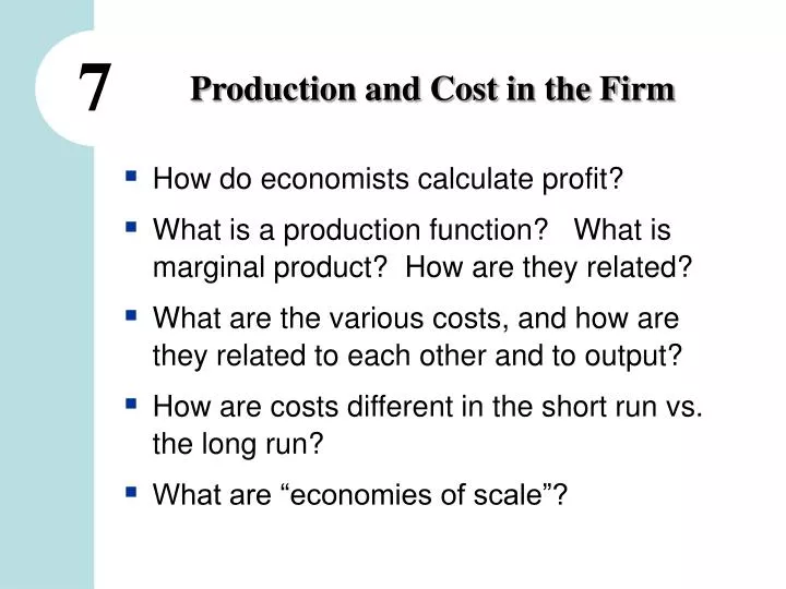
Production and Cost in the Firm. 7. How do economists calculate profit? What is a production function? What is marginal product? How are they related? What are the various costs, and how are they related to each other and to output?

E N D
Production and Cost in the Firm 7 • How do economists calculate profit? • What is a production function? What is marginal product? How are they related? • What are the various costs, and how are they related to each other and to output? • How are costs different in the short run vs. the long run? • What are “economies of scale”?
the amount a firm receives from the sale of its output the market value of the inputs a firm uses in production Total Revenue, Total Cost, Profit 0 • We assume that the firm’s goal is to maximize profit. Profit = Total revenue – Total cost
Costs: Explicit vs. Implicit 0 • Explicit costs – actual cash payments for resources, such as paying wages to workers • Implicit costs – opportunity cost of using owner-supplied resources, such as the opportunity cost of the owner’s time • Remember: The cost of something is the value of the next best alternative. • This is true whether the costs are implicit or explicit. Both matter for a firm’s decisions.
Explicit vs. Implicit Costs: An Example 0 Suppose you need $100,000 to start your business. The interest rate is 5%. • Case 1: borrow $100,000 • explicit cost = • Case 2: use $40,000 of your savings, borrow the other $60,000 • explicit cost = • implicit cost =
Economic Profit vs. Accounting Profit 0 • Accounting profit = total revenue minus total explicit costs • Economic profit = total revenue minus total costs (including BOTH explicit and implicit costs) • Accounting profit ignores implicit costs, so it will be greater than economic profit.
ACTIVE LEARNING 2: Economic profit vs. accounting profit The equilibrium rent on office space has just increased by $500 per month. Compare the effects on your firm’s accounting profit and economic profit if a. you rent your office space b. you own your office space 5
Production in the Short Run 0 • Some resources are considered to be variable and some are considered to be fixed. • It depends on how quickly the level can be altered to change the rate of output. • In the short run, at least one resource is fixed. • In the long run, all resources are variable.
The Production Function 0 • A production function shows the relationship between the quantity of inputs used to produce a good, and the quantity of output of that good. • It can be represented by a table, equation, or graph. • Example 1: • Farmer Jack grows wheat. • He has 5 acres of land. • He can hire as many workers as he wants.
L(# of workers) Q(bushels of wheat) 3,000 2,500 0 0 2,000 1 1,000 1,500 Quantity of output 2 1,800 1,000 3 2,400 500 4 2,800 0 0 1 2 3 4 5 5 3,000 # of workers EXAMPLE 1: Farmer Jack’s Production Function 0
∆Q ∆L Marginal Product 0 • The marginal productof any input is the increase in output arising from an additional unit of that input, holding all other inputs constant. • If Farmer Jack hires one more worker, his output rises by the marginal product of labor. • Marginal product of labor (MPL) =
L(# of workers) Q(bushels of wheat) 0 0 ∆Q = 1,000 ∆L = 1 1 1,000 ∆Q = 800 ∆L = 1 2 1,800 ∆L = 1 ∆Q = 600 3 2,400 ∆Q = 400 ∆L = 1 4 2,800 ∆L = 1 ∆Q = 200 5 3,000 EXAMPLE 1: Total & Marginal Product 0 MPL
3,000 2,500 2,000 Quantity of output 1,500 1,000 500 0 0 1 2 3 4 5 No. of workers EXAMPLE 1: MPL = Slope of Prod. Function 0 L(# of workers) Q(bushels of wheat) MPL MPL equals the slope of the production function. Notice that MPL diminishes as L increases. This explains why the production function gets flatter as L increases. 0 0 1,000 1 1,000 800 2 1,800 600 3 2,400 400 4 2,800 200 5 3,000
Why MPL Is Important • Recall from Chapter 1: Rational people choose actions for which the expected marginal benefit exceeds the expected marginal cost. • When Farmer Jack hires an extra worker, • his costs rise by the wage he pays the worker • his output rises by MPL • Comparing the wage and the change in his output helps Jack decide whether he would benefit from hiring the worker.
EXAMPLE 2: A “Fold-It” Factory We are going to create a factory that produces a product known as a “fold-it” • Resources: • factory • paper • stapler • staples • labor
Why MPL Diminishes • The Law of Diminishing Marginal Returns: the marginal product of a variable resource eventually falls as the quantity of the resource used increases (other things equal) • If we increases the # of workers but not the # of staplers or the desk area, each add’l worker has less to work with and will be less productive. • In general, MPL diminishes as L rises whether the fixed resource is land (as would be the case with Jack the wheat farmer) or capital (our desk and stapler).
EXAMPLE 1: Farmer Jack’s Costs • Farmer Jack must pay $1,000 per month for the land, regardless of how much wheat he grows. • The market wage for a farm worker is $2,000 per month. • So Farmer Jack’s costs are related to how much wheat he produces….
EXAMPLE 1: Farmer Jack’s Costs 0 L(# of workers) Q(bushels of wheat) Cost of land Cost of labor Total Cost 0 0 1 1,000 2 1,800 3 2,400 4 2,800 5 3,000
MC = ∆TC ∆Q Marginal Cost • Marginal Cost (MC) is the increase in Total Cost from producing one more unit:
Q(bushels of wheat) Total Cost 0 $1,000 ∆TC = $2000 ∆Q = 1000 1,000 $3,000 ∆TC = $2000 ∆Q = 800 1,800 $5,000 ∆TC = $2000 ∆Q = 600 2,400 $7,000 ∆TC = $2000 ∆Q = 400 2,800 $9,000 ∆TC = $2000 ∆Q = 200 3,000 $11,000 EXAMPLE 1: Total and Marginal Cost Marginal Cost (MC) $2.00 $2.50 $3.33 $5.00 $10.00
$2.00 $2.50 $3.33 $5.00 $10.00 EXAMPLE 1: The Marginal Cost Curve Q(bushels of wheat) TC MC MC usually rises as Q rises, as in this example. 0 $1,000 1,000 $3,000 1,800 $5,000 2,400 $7,000 2,800 $9,000 3,000 $11,000
Why MC Is Important • Farmer Jack is rational and wants to maximize his profit. To increase profit, should he produce more wheat or less? • To find the answer, Farmer Jack needs to “think at the margin.” • If the cost of an additional bushel of wheat (MC) is less than the revenue he would get from selling it, Jack’s profits rise if he produces more. (In the next chapter, we will learn more about how firms choose Q to maximize their profits.)
EXAMPLE 3 • Our third example is more general, and applies to any type of firm producing any good with any types of resources.
$100 $0 100 70 100 120 100 160 100 210 100 280 100 380 100 520 EXAMPLE 3:Costs 0 $800 FC Q FC VC TC VC $700 TC 0 $600 1 $500 2 Costs $400 3 $300 4 $200 5 $100 6 $0 7 0 1 2 3 4 5 6 7 Q
MC = ∆TC ∆Q EXAMPLE 3:Marginal Cost Recall, Marginal Cost (MC)is the change in total cost from producing one more unit: Q TC MC 0 $100 $70 1 170 50 2 220 40 3 260 Usually, MC rises as Q rises, due to diminishing marginal product. Sometimes (as here), MC falls before rising. (In other examples, MC may be constant.) 50 4 310 70 5 380 100 6 480 140 7 620
EXAMPLE 3: Average Fixed Cost 0 Average fixed cost (AFC)is fixed cost divided by the quantity of output: AFC = FC/Q Q FC AFC 0 $100 ---- 1 100 2 100 3 100 Notice that AFC falls as Q rises: The firm is spreading its fixed costs over a larger and larger number of units. 4 100 5 100 6 100 7 100
EXAMPLE 3:Average Variable Cost 0 Average variable cost (AVC)is variable cost divided by the quantity of output: AVC = VC/Q Q VC AVC 0 $0 ---- 1 70 2 120 3 160 As Q rises, AVC may fall initially. In most cases, AVC will eventually rise as output rises. 4 210 5 280 6 380 7 520
AFC AVC ---- ---- $100 $70 50 60 33.33 53.33 25 52.50 20 56.00 16.67 63.33 14.29 74.29 EXAMPLE 3:Average Total Cost 0 Average total cost (ATC) equals total cost divided by the quantity of output: ATC = TC/Q Q TC ATC 0 $100 1 170 2 220 3 260 Also, ATC = AFC + AVC 4 310 5 380 6 480 7 620
$200 $175 $150 $125 Costs $100 $75 $50 $25 $0 0 1 2 3 4 5 6 7 Q EXAMPLE 3:Average Total Cost 0 Q TC ATC Usually, as in this example, the ATC curve is U-shaped. 0 $100 ---- 1 170 $170 2 220 110 3 260 86.67 4 310 77.50 5 380 76 6 480 80 7 620 88.57
$200 $175 $150 AFC $125 AVC Costs $100 ATC $75 MC $50 $25 $0 0 1 2 3 4 5 6 7 Q EXAMPLE 3:The Cost Curves Together 0
ACTIVE LEARNING 3: Costs Fill in the blank spaces of this table. Q VC TC AFC AVC ATC MC 0 $50 ---- ---- ---- $10 1 10 $10 $60.00 2 30 80 30 3 16.67 20 36.67 4 100 150 12.50 37.50 5 150 30 60 6 210 260 8.33 35 43.33 30
$200 $175 $150 $125 Costs $100 $75 $50 $25 $0 0 1 2 3 4 5 6 7 Q EXAMPLE 3:Why ATC Is Usually U-shaped 0 As Q rises: Initially, falling AFCpulls ATC down. Eventually, rising AVCpulls ATC up.
$200 $175 $150 $125 Costs $100 ATC $75 MC $50 $25 $0 0 1 2 3 4 5 6 7 Q EXAMPLE 3:ATC and MC 0 When MC < ATC, ATC is falling. When MC > ATC, ATC is rising. The MC curve crosses the ATC curve at the ATC curve’s minimum.
Costs in the Long Run • Short run: Some inputs are fixed • Long run: All inputs are variable (firms can build new factories, or remodel or sell existing ones) • In the long run, ATC at any Q is cost per unit using the most efficient mix of inputs for that Q (the factory size with the lowest ATC).
Cost ($) ATCM ATCS ATCL Q EXAMPLE 4:LRAC with 3 Factory Sizes Firm can choose from 3 factory sizes: S, M, L. Each size has its own SRATC curve. The firm can change to a different factory size in the long run, but not in the short run.
Cost ($) ATCM ATCS ATCL Q QA QB EXAMPLE 4:LRAC with 3 Factory Sizes LRATC
Cost LRAC Q A Typical LRAC Curve In the real world, factories come in many sizes, each with its own SRATC curve. So a typical LRAC curve looks like this:
Cost LRAC Q How LRAC Changes as the Scale of Production Changes Economies of scale: LRAC falls as Q increases. Constant returns to scale: LRAC stays the same as Q increases. Diseconomies of scale: LRAC rises as Q increases.