Download
1 / 53
600 likes | 1.08k Views
Theory of the Firm: Production & Cost. A business firm is an organization, owned and operated by private individuals, that specializes in production Production is the process of combining inputs to make outputs

E N D
Theory of the Firm: Production & Cost • A business firm is an organization, owned and operated by private individuals, that specializes in production • Production is the process of combining inputs to make outputs • The firm buys inputs from households or other firms and sells its output to consumers • Profit of the firm = sales revenue – input costs
The Nature of the Firm • Every firm must deal with the government • Pays taxes to the government • Must obey government laws and regulations • Receive valuable services from the government • Public capital • Legal systems • Financial systems
Owners Initial Financing Profit After Taxes Input Costs Taxes Input Suppliers The Firm (Management) Government Inputs Government Services Government Regulations Output Revenue Customers Fig. 1 The Firm and Its Environment
Types of Business Firms • There are about 24 million business firms in United States—each of them falls into one of three legal categories • A sole proprietorship • A firm owned by a single individual • A partnership • A firm owned and usually operated by several individuals who share in the profits and bear personal responsibility for any losses • Both of the above face • Unlimited liability • Each owner is held personally responsible for the obligations of the firm • The difficulty of raising money to expand the business • Each partner bears full responsibility for the poor judgment of any one of them
Types of Business Firms • A corporation • Owned by those who buy shares of stock and whose liability is limited to the amount of their investment in the firm • Ownership is divided among those who buy shares of stock • Each share of stock entitles its owner to a share of the corporation’s profit • Some of this is paid out in dividends • If the corporation needs additional funds it may sell more stock • Offers the stockholder limited liability
Percent of Firms Percent of Total Sales Corporations 20% Partnerships 7% Corporations 90% SoleProprietorships 73% Partnerships 4% SoleProprietorships 6% Figure 2: Forms of Business Organization
Why a Firm? • Most firms have employees • People who work for a wage or salary, but are not themselves owners • Each worker could operate his own one-person firms as independent contractors • So why don’t more of us do this?
The Advantages of Employment • Gains from specialization • Lower transaction costs • Reduced risk
Further Gains From Specialization • Independent contractor must • Design the good • Make the good • Deal with customers • Advertise services • At a factory each of these tasks would be performed by different individuals who would work full time at their activity
Lower Transaction Costs • Transaction costs are time costs and other costs required to carry out market exchanges • In a firm with employees many supplies and services can be produced inside the organization • Firm can enjoy significant savings on transaction costs
Reduced Risk • Large firm with employees offers opportunities for everyone involved to reduce risk through • Diversification • Process of reducing risk by spreading sources of income among different alternatives • With large firms, two kinds of diversification are possible • Within the firm • Among firms • These advantages help it attract customers, workers, and potential owners
The Limits to the Firm • You might be tempted to conclude that bigger is always better • The larger the firm, the greater will be the cost savings • However, there are limits
Thinking About Production • Production involves using inputs to produce an output • Inputs include resources • Labor • Capital • Land • Raw materials • Other goods and services provided by other firms • Way in which these inputs may be combined to produce output is the firm’s technology
Production technology • A firm’s technology is treated as a given • Constraint on its production, which is spelled out by the firm’s production function • For each different combination of inputs, the production function tells us the maximum quantity of output a firm can produce over some period of time
Alternative Input Combinations Different Quantities of Output Production Function Figure 3: The Firm’s Production Function
The Short Run and the Long Run • Useful to categorize firms’ decisions into • Long-run decisions • Short-run decisions • To guide the firm over the next several years • Manager must use the long-run lens • To determine what the firm should do next week • Short run lens is best
Production in the Short Run • When firms make short-run decisions, there is nothing they can do about their fixed inputs • Fixed inputs • An input whose quantity must remain constant, regardless of how much output is produced • Variable input • An input whose usage can change as the level of output changes • Total product • Maximum quantity of output that can be produced from a given combination of inputs
Production in the Short Run • Marginal product of labor (MPL) is the change in total product (ΔQ) divided by the change in the number of workers hired (ΔL) • Tells us the rise in output produced when one more worker is hired, leaving all other inputs unchanged
Units of Output Number of Workers 1 6 2 4 3 5 Figure 4: Total and Marginal Product Total Product 196 184 161 DQ from hiring fourth worker 130 DQ from hiring third worker 90 DQ from hiring second worker 30 DQ from hiring first worker increasing marginal returns diminishing marginal returns
Marginal Returns To Labor • As more and more workers are hired • MPL first increases • Then decreases • Pattern is believed to be typical at many types of firms
Increasing Marginal Returns to Labor • When the marginal product of labor increases as employment rises, we say there are increasing marginal returns to labor • Each time a worker is hired, total output rises by more than it did when the previous worker was hired
Diminishing Returns To Labor • When the marginal product of labor is decreasing • There are diminishing marginal returns to labor • Output rises when another worker is added so marginal product is positive • But the rise in output is smaller and smaller with each successive worker • Law of diminishing (marginal) returns states that as we continue to add more of any one input (holding the other inputs constant) • Its marginal product will eventually decline
Costs • A firm’s total cost of producing a given level of output is the opportunity cost of the owners • Everything they must give up in order to produce that amount of output
The Irrelevance of Sunk Costs • Sunk cost is one that already has been paid, or must be paid, regardless of any future action being considered • Should not be considered when making decisions • Even a future payment can be sunk • If an unavoidable commitment to pay it has already been made
Explicit vs. Implicit Costs • Types of costs • Explicit (involving actual payments) • Money actually paid out for the use of inputs • Implicit (no money changes hands) • The cost of inputs for which there is no direct money payment
Costs in the Short Run • Fixed costs • Costs of a firm’s fixed inputs • Variable costs • Costs of obtaining the firm’s variable inputs
Measuring Short Run Costs: Total Costs • Types of total costs • Total fixed costs • Cost of all inputs that are fixed in the short run • Total variable costs • Cost of all variable inputs used in producing a particular level of output • Total cost • Cost of all inputs—fixed and variable • TC = TFC + TVC
Dollars $435 375 315 255 195 135 0 30 90 130 161 184 196 Units of Output Figure 5: The Firm’s Total Cost Curves TC TVC TFC TFC
Average Costs • Average fixed cost (AFC) • Total fixed cost divided by the quantity of output produced • Average variable cost (TVC) • Total variable cost divided by the quantity of output produced • Average total cost (TC) • Total cost divided by the quantity of output produced
Marginal Cost • Marginal Cost • Increase in total cost from producing one more unit or output • Marginal cost is the change in total cost (ΔTC) divided by the change in output (ΔQ) • Tells us how much cost rises per unit increase in output • Marginal cost for any change in output is equal to shape of total cost curve along that interval of output
Dollars $4 3 2 1 30 90 130 161 196 0 Units of Output Figure 6: Average And Marginal Costs MC AFC ATC AVC
Explaining the Shape of the Marginal Cost Curve • When the marginal product of labor (MPL) rises (falls), marginal cost (MC) ___ (___) • Since MPL ordinarily rises and then falls, MC will do the _____—it will ____ and then ______ • Thus, the MC curve is U-shaped
Average And Marginal Costs • At low levels of output, the MC curve lies below the AVC and ATC curves • These curves will slope downward • At higher levels of output, the MC curve will rise above the AVC and ATC curves • These curves will slope upward • As output increases; the average curves will first slope downward and then slope upward • Will have a U-shape • MC curve will intersect the minimum points of the AVC and ATC curves
Production And Cost in the Long Run • In the long run, there are no fixed inputs or fixed costs - All inputs and all costs are variable • The firm’s goal is to earn the highest possible profit • To do this, it must follow the least cost rule
Production And Cost in the Long Run • Long-run total cost • The cost of producing each quantity of output when the least-cost input mix is chosen in the long run • Long-run average total cost • The cost per unit of output in the long run, when all inputs are variable • The long-run average total cost (LRATC) • Cost per unit of output in the long-run
The Relationship Between Long-Run And Short-Run Costs • For some output levels, LRTC is smaller than TC • Long-run total cost can never be ____ than, short-run total cost (LRTC __ TC) • Long-run average cost can be never be ____ than the short–run average total cost (LRATC __ ATC)
Average Cost And Plant Size • Plant - Collection of fixed inputs at a firm’s disposal • In the long run, the firm can change the size of its plant • In the short run, it is stuck with its current plant size • ATC curve tells us how average cost behaves in the short run, when the firm uses a plant of a given size • To produce any level of output, it will always choose that ATC curve—among all of the ATC curves available—that enables it to produce at lowest possible average total cost
Graphing the LRATC Curve • A firm’s LRATC curve combines portions of each ATC curve available to firm in the long run • In the short run, a firm can only move along its current ATC curve • In the long run it can move from one ATC curve to another by varying the size of its plant
Dollars $4.00 3.00 2.00 1.00 30 90 130 161 184 250 300 0 196 Units of Output Figure 7: Long-Run Average Total Cost ATC1 LRATC ATC3 ATC0 ATC2 C D B E A 175 Use 0 automated lines Use 1 automated lines Use 2 automated lines Use 3 automated lines
Economies of Scale • Economics of scale • Long-run average age total cost _______ as output increases • When an increase in output causes LRATC to ______, we say that the firm is enjoying economies of scale • When long-run total cost rises proportionately less than output, production is characterized by economies of scale • LRATC curve slopes downward
Dollars $4.00 3.00 2.00 1.00 130 184 Figure 8: The Shape Of LRATC LRATC 0 Economies of Scale Constant Returns to Scale Diseconomies of Scale Units of Output
Gains From Specialization • One reason for economies of scale is gains from specialization • Opportunities for increased specialization occur at lower levels of output • With a relatively small plant and small workforce
More Efficient Use of Lumpy Inputs • Economies of scale involves the “lumpy” nature of many types of plant and equipment • Plant and equipment must be purchased in large lumps • Making more efficient use of lumpy inputs will have more impact on LRATC at low levels of output • When these inputs make up a greater proportion of the firm’s total costs
Diseconomies of Scale • Long-run average total cost _______ as output increases • As output continues to increase, most firms will reach a point where bigness begins to cause problems • When long-run total cost rises more than in proportion to output, there are diseconomies of scale • LRATC curve slopes upward • Diseconomies of scale are more likely at higher output levels
Constant Returns To Scale • Long-run average total cost ___ _________ as output increases • When both output and long-run total cost rise by the same proportion, production is characterized by constant returns to scale • LRATC curve is flat
In sum… • The LRATC, often shows the following pattern • Economies of scale (decreasing LRATC) at relatively low levels of output • Constant returns to scale (constant LRATC) at some intermediate levels of output • Diseconomies of scale (increasing LRATC) at relatively high levels of output • This is why LRATC curves are typically U-shaped
Long Run Costs, Market Structure and Mergers • The number of firms in a market determines the market structure • What accounts for these differences in the number of sellers in the market? • Shape of the LRATC curve plays an important role in the answer
LRATC and the Size of Firms • The output level at which the LRATC first hits bottom is known as the minimum efficient scale (MES) for the firm • Lowest level of output at which it can achieve minimum cost per unit • Can also determine the maximum possible total quantity demanded by using market demand curve • Applying these two curves—the LRATC for the typical firm, and the demand curve for the entire market—to market structure • When the MES is small relative to the maximum potential market • Firms that are relatively small will have a cost advantage over relatively large firms • Market should be populated by many small firms, each producing for only a tiny share of the market
LRATC and the Size of Firms • There are significant economies of scale that continue as output increases • Even to the point where a typical firm is supplying the maximum possible quantity demanded • This market will gravitate naturally toward monopoly • In some cases the MES occurs at 25% of the maximum potential market • In this type of market, expect to see a few large competitors • There are significant lumpy inputs that create economies of scale • Until each firm has expanded to produce for a large share of the market
Dollars $160 80 1,000 3,000 100,000 0 Units per Month Figure 9: How LRATCHelps Explain Market Structure LRATCTypical Firm F E DMarket