Download
1 / 31
310 likes | 314 Views
This study group will cover topics such as game tree evaluation, lower bounds on running time, introduction to game theory, and the use of randomized algorithms. Join us on June 21st to learn more!

E N D
Study GroupRandomized Algorithms 21st June 03
Topics Covered • Game Tree Evaluation • its expected run time is better than the worst-case complexity of any deterministic algorithm • demonstrates a technique to derive a lower bound on running time of any randomized algorithm for a problem • Introduction to Game Theory • leads to the Minimax Principle
Definition of Game Tree • a Game Tree Td,k is uniform tree in which the root and the internal nodes has d children and every leaf is at distance 2k from the root • internal nodes at even distance from the root are labeled MIN and at odd distance are labeled MAX • each leaf is associated with a value
MIN MAX MAX MIN MIN MIN MIN MAX MAX MAX MAX MAX MAX MAX MAX 0 1 0 0 0 1 0 1 0 1 0 0 0 1 0 1 Example of a Game Tree T2,2
Observations • Every root-to-leaf path goes through the same number of MIN and MAX nodes (including the root) • If the depth of the tree is 2k, there are 22k = 4k leaves
1 0 0 0 MIN MIN MIN MIN 1 0 1 0 1 1 0 0 Game Tree Evaluation • MIN (AND) Node • returns the lesser of the two children
1 0 1 1 MAX MAX MAX MAX 1 1 0 0 1 0 0 1 Game Tree Evaluation • MAX (OR) Node • returns the greater of the two children
AND OR OR AND AND AND AND OR OR OR OR OR OR OR OR 0 1 0 0 0 1 0 1 0 1 0 0 0 1 0 1 What is the value returned by the root?
AND AND OR OR OR OR 0 1 0 1 0 1 1 0 a better case – visit 2 leaves is enough worst case – need to visit ALL 4k leaves A Deterministic Algorithm • Depth-first manner • always visit the left child before the right child
AND OR OR 0 1 0 1 Expected cost (number of leaves visited) 3 A Randomized Algorithm • Coin toss • 0.5 probability choosing the left child and 0.5 probability choosing the right child
Design Rationale • Suppose AND node were to return 0 • at least one of the leaves is 0 • if deterministic algorithm is used, your opponent can always “hide” this 0 and make your algorithm visit both leaves • if randomized algorithm is used, you foils your opponent’s strategy. The expected number of steps (leaf visits) is 3/2 • Similar for OR node were to return 1
Design Rationale • Expected cost • EAND_0 = EOR_1 = 3/2 • What if AND(OR) node were to return 1(0)? • both children are 1(0), it seems that the randomized algorithm doesn’t improve much since we need to visit both children anyway • however, it benefits the parent level
Analysis of the Randomized Algo. • Claim: The expected cost of the randomized algorithm for evaluating any T2,k game tree is at most 3k • Proof by induction: • consider k = 1 • expected cost 3
AND return 0 OR OR 0 0 0 1 Analysis of the Randomized Algo. • Case I – root evaluated to 0 • at least one of the subtrees (OR nodes) gives 0 • you have 0.5 probability that this particular node is checked first • E(T) = ½ 2 + ½ (3/2 + 2) = 2.75
return 1 AND OR OR 0 1 0 1 Analysis of the Randomized Algo. • Case II – root evaluated to 1 • both subtrees give 1 • E(T) = 2 3/2 = 3 • Both cases give 3 expected cost, so the claim is true for k=1
either gives 1 or 0 OR T2,k-1 T2,k-1 Analysis of the Randomized Algo. • Assume that for all T2,k-1, the expected cost 3k-1 • First, consider the OR-root tree
either 1 or 0 OR T2,k-1 T2,k-1 Analysis of the Randomized Algo. • Case I: OR-root gives 1 • at least one subtree gives 1 • 0.5 probability we use it first • E(T) ½ 3k-1 + ½ 2 3k-1 = 3/2 3k-1 • Case II: OR-root gives 0 • both subtrees give 0 • E(T) 2 3k-1
T2,k OR OR OR AND T2,k-1 T2,k-1 T2,k-1 T2,k-1 T2,k-1 T2,k-1 Analysis of the Randomized Algo. • Now, consider the AND-root game tree, T2,k
either 1 or 0 OR OR AND T2,k-1 T2,k-1 T2,k-1 T2,k-1 Analysis of the Randomized Algo. • Case I: AND-root gives 0 • at least one subtree gives 0 • 0.5 probability we use it first • E(T2,k) ½ 2 3k-1 + ½ (3/2 3k-1 + 2 3k-1) = 2.75 3k-1 3k • Case II: AND-root gives 1 • both subtrees give 1 • E(T2,k) 2 3/2 3k-1 = 3k
Analysis of the Randomized Algo. • Proved the claim: The expected cost of the randomized algorithm for evaluating any T2,k game tree is at most 3k • A tree has n = 4k leaves, then k = log4n. Substitute log4n for k in the expected cost, then the cost 3log4n. By xlogab = blogax, the cost nlog43 =n0.793
Question Our randomized algorithm for the game tree evaluation of any uniform binary tree with n leaves is n0.793. Can we establish that no randomized algorithm can have a lower expected running time? YES! Using Yao’s technique the Minimax Theorem Game Theory Basics
Introduction to Game Theory • Consider the stone-paper-scissors game between 2 players • loser pays $1 to the winner • payoff matrix M : Mij denotes the payoff by the Column player to the Row player
Two-person Zero-sum Game • Zero-sum game • the net amount won by C and R is exactly zero, i.e., the amount of money is not increased or decreased among them • Every two-person zero-sum game can be represented by a nm payoff matrix
Pure Strategy v.s. Mixed Strategy • Pure (Deterministic) strategy • always uses the same strategy or a deterministic pattern, e.g., R always chooses ‘stone’ while C always chooses ‘paper’ • Mixed (Randomized) strategy • the strategy chosen by a player is randomized, i.e., a probability distribution among all possible strategies
Pure Optimal Strategy • Zero-information game • the strategy chosen by the opponent is unknown • Naturally, the goal of the row (column) player is to maximize (minimize) the payoff • If R chooses strategy i, then she is guaranteed a payoff of minjMij, regardless of what C’s strategy is • Optimal strategy for R is an strategy i that maximize minjMij.
Pure Optimal Strategy • Similarly, the optimal strategy of C is • If C chooses strategy j, then he is guaranteed a loss of no more than maxiMij, regardless of what R’s strategy is • Optimal strategy for C is an strategy j that minimize maxiMij. • Let Vr = maximinjMij and Vc = minjmaxiMij be the lower bound of payoff R can get and the upper bound of loss C can ensure respectively
j Vr z i Vc Clearly, Vr z Vc Inequality for All Payoff Matrix • Minimax Inequality maximinjMijminjmaxiMij • Proof:
Saddle-point • If Vr = Vc, we say the game has a solution and the value of the game is V = Vr = Vc • the solution is also known as the saddle-point of the game • If no saddle-point exists, it means there is no clear-cut pure optimal strategy for any player
Mixed Strategy Game • The Row player picks a vector p = (p1, …, pn), which is a probability distribution on the rows of M. (i.e., pi is the probability that R will choose strategy i) • Similarly, the Column player picks a vector q = (q1, …, qm), i.e., qj is the probability that R will choose strategy j)
Mixed Optimal Strategy • Expected Payoff • E[payoff] = pT M q • R aims to maximize it while C aims to minimizes it • As before, let Vr = maxpminqpT M q be the lower bound of the expected payoff R can get using a strategy p • Let VC = minqmaxppT M q be the upper bound of the expected payoff C need to pay using a strategy q
von Neumann’s Mininmax Theorem • For any two person, zero-sum game specified by a matrix M maxpminqptMq = minqmaxppTMq • the optimal strategy for R will yield the same payoff as the optimal strategy for C! • if either player uses his optimal strategy, the opponent cannot improve the payoff