Download
1 / 31
350 likes | 625 Views
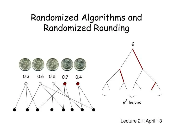
Randomized Algorithms and Randomized Rounding. G. Lecture 21: April 13. 0.3. 0.6. 0.2. 0.7. 0.4. n 2 leaves. Minimum Cut. A cut is a set of edges whose removal disconnects the graph. Minimum cut : Given an undirected multigraph G with n vertices,

E N D
Randomized Algorithms and Randomized Rounding G Lecture 21: April 13 0.3 0.6 0.2 0.7 0.4 n2 leaves
Minimum Cut A cut is a set of edges whose removal disconnects the graph. Minimum cut: Given an undirected multigraph G with n vertices, find a cut of minimum cardinality (a min-cut). This problem can be solved in polynomial by the max-flow algorithm. However, using randomness, we can design a really simple algorithm.
Edge Contraction 5 5 1 4 4 3 3 2 1,2 Contraction of an edge e = (u,v): Merge u and v into a single vertex “uv”. For any edge (w,u) or (w,v), this edge becomes (w,“uv”) in the resulting graph. Delete any edge which becomes a “self-loop”, i.e. an edge of the form (v,v).
Edge Contraction 5 5 1 4 4 3 3 2 1,2 Observation: an edge contraction would not decrease the min-cut size. This is because every cut in the graph at any intermediate stage is a cut in the original graph.
A Randomized Algorithm Running time: Each iteration takes O(n) time. Each iteration has one fewer vertices. So, there are at most n iteration. Total running time O(n2). • Algorithm Contract: • Input: A multigraph G=(V,E) • Output: A cut C • H <- G. • while H has more than 2 vertices do • 2.1 choose an edge (x,y) uniformly at random from the edges in H. • 2.2 H <- H/(x,y). (contract the edge (x,y)) • 3. C <- the set of vertices corresponding to one of the two meta-vertices in H.
Analysis Obviously, this algorithm will not always work. How should we analyze the success probability? Let C be a minimum cut, and E(C) be the edges crossing C. Claim 1: C is produced as output if and only if none of the edges in E(C) is contracted by the algorithm. So, we want to estimate the probability that an edge in E(C) is picked. What is this probability?
Analysis Let k be the number of edges in E(C). How many edges are there in the initial graph? Claim 2: The graph has at least nk/2 edges. Because each vertex has degree at least k. So, the probability that an edge in E(C) is picked at the first iteration is at most 2/n.
Analysis In the i-th iteration, there are n-i+1 vertices in the graph. Observation: an edge contraction would not decrease the min-cut size. So the min-cut still has at least k edges. Hence there are at least (n-i+1)k/2 edges in the i-th iteration. The probability that an edge in E(C) is picked is at most 2/(n-i+1).
Analysis So, the probability that a particular min-cut is output by Algorithm Contract with probability at least Ω(n-2).
Boosting the Probability To boost the probability, we repeat the algorithm for n2log(n) times. What is the probability that it still fails to find a min-cut? So, high probability to find a min-cut in O(n4log(n)) time.
Ideas to an Improved Algorithm Key: The probability that an edge in E(C) is picked is at most 2/(n-i+1). Observation: at early iterations, it is not very likely that the algorithm fails. Idea: “share” the random choices at the beginning! In the previous algorithm, we boost the probability by running the Algorithm Contract (from scratch) independently many times. G n contractions n2 leaves
Ideas to an Improved Algorithm Idea: “share” the random choices at the beginning! G G n/2 contractions n contractions n/4 contractions ……………… n/8 contractions n2 leaves n2 leaves Previous algorithm. New algorithm. log(n) levels
A Fast Randomized Algorithm • Algorithm FastCut: • Input: A multigraph G=(V,E) • Output: A cut C • n <- |V|. • if n <= 6, then compute min-cut by brute-force enumeration else • 2.1 t <- (1 + n/√2). • 2.2 Using Algorithm Contract, perform two independent contraction sequences to obtain graphs H1 and H2 each with t vertices. • 2.3 Recursively compute min-cuts in each of H1 and H2. • 2.4 return the smaller of the two min-cuts.
A Surprise Theorem 1: Algorithm Fastcut runs in O(n2 log(n)) time. Theorem 2: Algorithm Fastcut succeeds with probability Ω(1/log(n)). By a similar boosting argument, repeating Fastcut for log2(n) times would succeed with high probability. Total running time = O(n2 log3(n))! It is much faster than the best known deterministic algorithm, which has running time O(n3). Min-cut is faster than Max-Flow!
Complexity Theorem 1: Algorithm Fastcut runs in O(n2 log(n)) time. Formal Proof: Let T(n) be the running time of Fastcut when given an n-vertex graph. And the solution to this recurrence is: Q.E.D.
Complexity G n/2 contractions n/4 contractions log(n) levels n/8 contractions n2 leaves First level complexity = 2 x (n2/2) = n2. Second level complexity = 4 x (n2/4) = n2. Total time = n2 log(n). The i-th level complexity = 2i x (n2/2i) = n2.
Analysis Theorem 2: Algorithm Fastcut succeeds with probability Ω(1/log(n)). G n/2 contractions n/4 contractions log(n) levels n/8 contractions n2 leaves Claim: for each “branch”, the survive probability is at least ½.
Analysis Claim: for each “branch”, the survive probability is at least ½.
Analysis Theorem 2: Algorithm Fastcut succeeds with probability Ω(1/log(n)). Proof: Let k denote the depth of recursion, and p(k) be a lower bound on the success probability. For convenience, set it to be equality:
Analysis Theorem 2: Algorithm Fastcut succeeds with probability Ω(1/log(n)). We want to prove that p(k) = Ω(1/k), and then substituting k=log(n) would do. It is more convenient to replace p(k) by q(k) = 4/p(k)-1, and we have: A simple inductive argument now establishes that So q(k) = O(k) where
Remarks Fastcut is fast, simple and cute. Just for fun: A randomized algorithm for minimum k-cut with running time O(nf(k))? Open question 1: A deterministic algorithm for min-cut with running time close to O(n2)? Open question 2: A randomized algorithm for min-cut with running time close to O(m)? Open question 3: Is minimum cut really easier than maximum flow?
Set Cover Set cover problem: Given a ground set U of n elements, a collection of subsets of U, S* = {S1,S2,…,Sk}, where each subset has a cost c(Si), find a minimum cost subcollection of S* that covers all elements of U. Vertex cover is a special case, why? A convenient interpretation: sets elements Choose a min-cost set of white vertices to “cover” all black vertices.
Linear Programming Relaxation for each element e. for each subset S. How to “round” the fractional solutions? Idea: View the fractional values as probabilities, and do it randomly!
Algorithm First solve the linear program to obtain the fractional values x*. Then flip a (biased) coin for each set with probability x*(S) being “head”. 0.3 0.6 0.2 0.7 0.4 sets elements Add all the “head” vertices to the set cover. Repeat log(n) rounds.
Performance Theorem: The randomized rounding gives an O(log(n))-approximation. Claim 1: The sets picked in each round have an expected cost of at most LP. Claim 2: Each element is covered with high probability after O(log(n)) rounds. So, after O(log(n)) rounds, the expected total cost is at most O(log(n)) LP, and every element is covered with high probability, and hence the theorem. Remark: It is NP-hard to have a better than O(log(n))-approximation!
Cost Claim 1: The sets picked in each round have an expected cost of at most LP. Q.E.D.
Feasibility Claim 2: Each element is covered with high probability after O(log(n)) rounds. First consider the probability that an element e is covered after one round. Let say e is covered by S1, …, Sk which have values x1, …, xk. By the linear program, x1 + x2 + … + xk >= 1. Pr[e is not covered in one round] = (1 – x1)(1 – x2)…(1 – xk). This is maximized when x1=x2=…=xk=1/k, why? Pr[e is not covered in one round] <= (1 – 1/k)k
Feasibility Claim 2: Each element is covered with high probability after O(log(n)) rounds. First consider the probability that an element e is covered after one round. Pr[e is not covered in one round] <= (1 – 1/k)k So, What about after O(log(n)) rounds?
Feasibility Claim 2: Each element is covered with high probability after O(log(n)) rounds. So, So,
Remark Let say the sets picked have an expected total cost of at most clog(n) LP. Claim: The total cost is greater than 4clog(n) LP with probability at most ¼. This follows from the Markov inequality, which says that: Proof of Markov inequality: The claim follows by substituting E[X]=clog(n)LP and t=4clog(n)LP
Wrap Up Theorem: The randomized rounding gives an O(log(n))-approximation. This is the only known rounding method for set cover. Randomized rounding has many other applications.