Download
1 / 39
440 likes | 801 Views
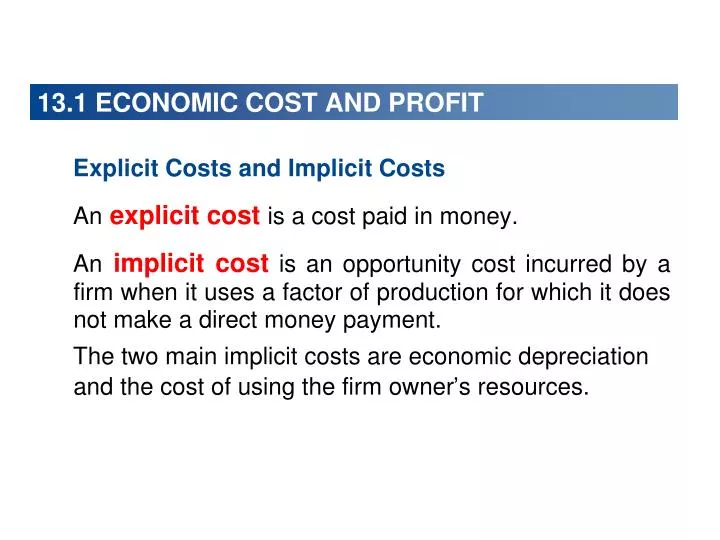
13.1 ECONOMIC COST AND PROFIT. Explicit Costs and Implicit Costs An explicit cost is a cost paid in money. An implicit cost is an opportunity cost incurred by a firm when it uses a factor of production for which it does not make a direct money payment.

E N D
13.1 ECONOMIC COST AND PROFIT • Explicit Costs and Implicit Costs • An explicit costis a cost paid in money. • An implicit cost is an opportunity cost incurred by a firm when it uses a factor of production for which it does not make a direct money payment. • The two main implicit costs are economic depreciation and the cost of using the firm owner’s resources.
13.1 ECONOMIC COST AND PROFIT • Economic depreciation is an opportunity cost of a firm using capital that it owns—measured as the change in the market value of capital over a given period. • Normal profitis the return to entrepreneurship. • Normal profit is part of a firm’s opportunity cost because it is the cost of the entrepreneur not running another firm.
13.1 ECONOMIC COST AND PROFIT • Economic Profit • A firm’s economic profit equals total revenue minus total cost. • Total cost is the sum of the explicit costs and implicit costs and is the opportunity cost of production. • Because the firm’s implicit costs is normal profit, the return to the entrepreneur equals normal profit plus economic profit. • If a firm incurs an economic loss, the entrepreneur receives less than normal profit.
13.1 ECONOMIC COST AND PROFIT Figure 13.1 shows two views of cost and profit. Total revenue equals price multiplied by quantity sold. Economists measure economic profit as total revenue minus opportunity cost.
13.1 ECONOMIC COST AND PROFIT • Opportunity cost is the sum of • explicit costs and • implicit cost (including normal profit).
13.1 ECONOMIC COST AND PROFIT Accountants measure cost as the sum of explicit costs and accounting depreciation. Accounting profit is total revenue minus accounting costs.
SHORT RUN AND LONG RUN • The Short Run: Fixed Plant • The short run is a time frame in which the quantities of some resources are fixed. • In the short run, a firm can usually change the quantity of labor it uses but not the quantity of capital. • The Long Run: Variable Plant • The long run is a time frame in which the quantities of all resources can be changed. • A sunk cost is irrelevant to the firm’s decisions.
13.3 SHORT-RUN COST • To produce more output in the short run, a firm employs more labor, which means the firm must increase its costs. • We describe the relationship between output and cost using three cost concepts: • Total cost • Marginal cost • Average cost
13.3 SHORT-RUN COST • Total Cost • A firm’s total cost (TC) is the cost of all the factors of production the firm uses. • Total cost divides into two parts: • Total fixed cost (TFC) is the cost of a firm’s fixed factors of production used by a firm—the cost of land, capital, and entrepreneurship. • Total fixed cost doesn’t change as output changes.
13.3 SHORT-RUN COST • Total variable cost (TVC) is the cost of the variable factor of production used by a firm—the cost of labor. • To change its output in the short run, a firm must change the quantity of labor it employs, so total variable cost changes as output changes. • Total cost is the sum of total fixed cost and total variable cost. That is, • TC = TFC + TVC • Table 13.2 on the next slide shows Sam’s Smoothies’ costs.
13.3 SHORT-RUN COST Figure 13.5 shows Sam’s Smoothies’ total cost curves. Total fixed cost (TFC) is constant—it graphs as a horizontal line. Total variable cost (TVC) increases as output increases. Total cost (TC) also increases as output increases.
13.3 SHORT-RUN COST The vertical distance between the total cost curve and the total variable cost curve is total fixed cost, as illustrated by the two arrows.
13.3 SHORT-RUN COST • Marginal Cost • A firm’s marginal cost is the change in total cost that results from a one-unit increase in total product. • Marginal cost tells us how total cost changes as total product changes. • Table 13.3 on the next slide calculates marginal cost for Sam’s Smoothies.
13.3 SHORT-RUN COST • Average Cost • There are three average cost concepts: • Average fixed cost (AFC) is total fixed cost per unit of output. • Average variable cost (AVC) is total variable cost per unit of output. • Average total cost (ATC) is total cost per unit of output.
TC = TFC + TVC Q Q Q 13.3 SHORT-RUN COST • The average cost concepts are calculated from the total cost concepts as follows: TC = TFC + TVC • Divide each total cost term by the quantity produced, Q, to give or, ATC = AFC + AVC
13.3 SHORT-RUN COST Figure 13.6 shows average cost curves and marginal cost curve at Sam’s Smoothies. Average fixed cost (AFC) decreases as output increases. The average variable cost curve (AVC) is U-shaped. The average total cost curve (ATC) is also U-shaped.
13.3 SHORT-RUN COST The vertical distance between these two curves is equal to average fixed cost, as illustrated by the two arrows. The marginal cost curve (MC) is U-shaped and intersects the average variable cost curve and the average total cost curve at their minimum points.
13.3 SHORT-RUN COST • Why the Average Total Cost Curve Is U-Shaped • Average total cost, ATC, is the sum of average fixed cost, AFC, and average variable cost, AVC. • The shape of the ATC curve combines the shapes of the AFC and AVC curves. • The U shape of the average total cost curve arises from the influence of two opposing forces: • Spreading total fixed cost over a larger output • Decreasing marginal returns
13.3 SHORT-RUN COST • Cost Curves and Product Curves • The technology that a firm uses determines its costs. • At low levels of employment and output, as the firm hires more labor, marginal product and average product rise, and marginal cost and average variable cost fall. • Then, at the point of maximum marginal product, marginal cost is a minimum. • As the firm hires more labor, marginal product decreases and marginal cost increases.
13.3 SHORT-RUN COST • But average product continues to rises, and average variable cost continues to fall. • Then, at the point of maximum average product, average variable cost is a minimum. • As the firm hires even more labor, average product decreases and average variable cost increases.
13.3 SHORT-RUN COST Figure 13.7 illustrates the relationship between the product curves and cost curves. A firm’s marginal cost curve is linked to its marginal product curve. If marginal product rises, marginal cost falls. If marginal product is a maximum, marginal cost is a minimum.
13.3 SHORT-RUN COST A firm’s average variable cost curve is linked to its average product curve. If average product rises, average variable cost falls. If average product is a maximum, average variable cost is a minimum.
13.3 SHORT-RUN COST At small outputs, MP and AP rise and MC and AVC fall. At intermediate outputs, MP falls and MC rises and AP rises and AVC falls. At large outputs, MP and AP fall and MC and AVC rise.
13.3 SHORT-RUN COST • Shifts in Cost Curves • Technology • A technological change that increases productivity shifts the total product curve upward. It also shifts the marginal product curve and the average product curve upward. • With a better technology, the same inputs can produce more output, so an advance in technology lowers the average and marginal costs and shifts the short-run cost curves downward.
13.3 SHORT-RUN COST Prices of Factors of Production • An increase in the price of a factor of production increases costs and shifts the cost curves. • But how the curves shift depends on which resource price changes. An increase in rent or another component of fixed cost • Shifts the fixed cost curves (TFC and AFC) upward. • Shifts the total cost curve (TC) upward. • Leaves the variable cost curves (AVC and TVC) and the marginal cost curve (MC) unchanged.
13.3 SHORT-RUN COST • An increase in the wage rate or another component of variable cost • Shifts the variable curves (TVC and AVC) upward. • Shifts the marginal cost curve (MC) upward. • Leaves the fixed cost curves (AFC and TFC) unchanged.
13.4 LONG-RUN COST • Plant Size and Cost • When a firm changes its plant size, its cost of producing a given output changes. • Will the average total cost of producing a gallon of smoothie fall, rise, or remain the same? • Each of these three outcomes arise because when a firm changes the size of its plant, it might experience: • Economies of scale • Diseconomies of scale • Constant returns to scale
13.4 LONG-RUN COST • Economies of Scale • Economies of scale exist if when a firm increases its plant size and labor employed by the same percentage, its output increases by a larger percentage and average total cost decreases. • The main source of economies of scale is greater specialization of both labor and capital.
13.4 LONG-RUN COST • Diseconomies of Scale • Diseconomies of scale exist if when a firm increases its plant size and labor employed by the same percentage, its output increases by a smaller percentage and average total cost increases. • Diseconomies of scale arise from the difficulty of coordinating and controlling a large enterprise. • Eventually, management complexity brings rising average total cost.
13.4 LONG-RUN COST • Constant Returns to Scale • Constant returns to scale exist if when a firm increases its plant size and labor employed by the same percentage, its output increases by the same percentage and average total cost remains constant. • Constant returns to scale occur when a firm is able to replicate its existing production facility including its management system.
13.4 LONG-RUN COST • The Long-Run Average Cost Curve • The long-run average cost curve shows the lowest average cost at which it is possible to produce each output when the firm has had sufficient time to change both its plant size and labor employed.
13.4 LONG-RUN COST Figure 13.8 shows a long-run average cost curve. In the long run, Sam’s Smoothies can vary both capital and labor inputs. With its current plant, Sam’s ATC curve is ATC1. With successively larger plants, Sam’s ATC curves would be ATC2,ATC3,and ATC4.
13.4 LONG-RUN COST The long-run average cost curve, LRAC, traces the lowest attainable average total cost of producing each output.
13.4 LONG-RUN COST Sam’s experiences economies of scale as output increases to 9 gallons an hour, … constant returns to scale for outputs between 9 gallons and 12 gallons an hour, … and diseconomies of scale for outputs that exceed 12 gallons an hour.