Download
1 / 1
10 likes | 90 Views
This innovative CO2 forecast product provides real-time data globally using ECMWF's Integrated Forecasting System, assessing atmospheric CO2 abundance variations accurately. Evaluations highlight discrepancies for further enhancement.

E N D
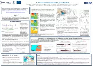
P1: A new real-time atmospheric CO2 forecast product Anna Agusti-Panareda1,SebastienMassart1, Gianpaolo Balsamo1, Anton Beljaars1, Souhail Boussetta1, Frederic Chevallier2, Richard J. Engelen1 1European Centre for Medium range Weather Forecasts, Reading, UK, 2Laboratoire des Sciences du Climat et l'Environnement, Gif-sur-Yvette, France • Evaluation of the CO2forecast MACC-II has recently started producing forecasts of atmospheric CO2 abundance using the infrastructure of the European Centre for Medium range Weather Forecasts (ECMWF) Integrated Forecasting System (IFS). The CO2 forecasts are provided globally in near-real-time since October 2012 with a five-day lead time: http://www.gmes-atmosphere.eu/d/services/gac/nrt/nrt_fields_co2 The phase and amplitude of the CO2 seasonal cycle vary with latitude. The model is evaluated using the NOAA GLOBALVIEW-CO2 (2011) dataset which provides the integrated effects of surface CO2 fluxes over large regions at different latitudinal bands. At first glance, the seasonal cycle phase and amplitude and latitude dependence shown in Figure 3 appear to be reasonably well represented in the forecast. However, there are clear discrepancies between the forecast and GLOBALVIEW-CO2 product in the northern hemisphere: ♦ In the forecast, not enough CO2 is released before and after the growing season (i.e. March to May and October to December). ♦The onset of the CO2 sink associated with the growing season starts too early in the forecast (e.g. the sharp CO2 decrease in mid-latitudes depicted by GLOBALVIEW-CO2 product in June starts in May in the forecast). This also leads to a longer growing season in the forecast. The combination of these two factors is consistent with the predominantly negative global annual bias shown in Figure 2. MACC-II Figure 4: (a) CO2 dry molar fraction anomalies [ppm]. Areas above 392ppm at 10-m level (grey), and at 850 hPa level (cyan), and areas above 388ppm level at 500 hPa level and 300 hPa level. Black contours depict mean seal level pressure and the location of Park Falls is marked by red triangle. (b) ECMWF surface pressure forecast [hPa].(c) Daily mean CO2 dry molar fraction [ppm] from the 24-hour forecast in cyan and observations in black at the top level (396m) of the NOAA/ESRL tall tower at Park Falls (Winsconsin, USA) in September 2010 (Andrews et al., 2013, Atmos. Meas. Tech. Discuss., 6, 1461-1553). • The pre-operational Monitoring of Atmospheric Composition and Climate - Interim Implementation service (MACC-II, http://www.gmes-atmosphere.eu/) provides data records on atmospheric composition for recent years, data for monitoring present conditions and forecasts of the distribution of key constituents for a few days ahead. The forecast configuration • The CO2 forecast relies on prescribed and modelled CO2 fluxes as well as the transport from the IFS model. • The IFS transport model is the state-of-the-art Numerical Weather Prediction (NWP) model from ECMWF. It has a semi-lagrangian advection scheme, a mass flux convection scheme and a turbulence mixing scheme. • The synoptic variability of CO2 associated with the passage of low pressure systems is well captured by the forecast . Figures 3 and 4 illustrate this at the NOAA/ESRL tall tower in Park Falls (Winsconsin, USA)in September 2010. • The cloudy warm conveyor belts in the mid-latitude low pressure systems are associated with changes in temperature and solar radiation at the surface which in turn increase the net ecosystem exchange. This increase can be linked with the following: • A decrease in the photosynthetic uptake following a decrease in radiation (e.g. 3 and 7 September) • An increase in ecosystem respiration following an increase in temperature (e.g. 21 September) • Both, a simultaneous decrease in the vegetation uptake and increase in ecosystem respiration due to a concurrent decrease in radiation and increase in temperature (e.g. 11 and 23 to 24 September) Figure 5: (a) Daily mean biogenic fluxes: net ecosystem exchange in cyan, photosynthetic uptake in green and ecosystem respiration in red [kg m-2 s-1]. (b) Daily mean 2-metre temperature [K]. (c) Daily mean downward solar radiation at the surface [J m-2] from the 24-hour forecast at Park Falls in September 2010. Figure 1: Set up of real time CO2 forecast Figure 3: NOAA-GLOBALVIEW CO2 product for 2010 based on observations, (b) equivalent product based on the 24 hour forecast of CO2 and (c) the difference between GLOBALVIEW and the forecast. The CO2 forecast has been sampled at the same locations as the GLOBALVIEW observations and the same data processing described in Masarie and Tans (1995, J.Geophys. Res., 100, 11593-11610) has been applied. • Thanks to the CTESSEL Carbon module development in the IFS, as part of the Geoland-2 project (http://www.gmes-geoland.info/), the net ecosystem exchange (NEE) is now available in near-real-time (Boussetta et al., 2012). The biomass burning fluxes from the MACC-II Global Fire Assimilation System (GFAS) are also used in near-real-time (Kaiser et al., 2012). The ocean fluxes are from the Takahashi et al. (2009) climatology . The anthropogenic emissions are from the EDGARv4.2 inventory (http://edgar.jrc.ec.europa.eu/) with an extrapolation of the last year available (2008) based on a climatology of its global trend . • The forecast is run at two resolutions: the resolution of ERA-Interim (T255,~77km, L60) and the resolution of the operational NWP model (T1279,~16 km, L91). • As there are no CO2 observations used in the forecast, the global budget is not constrained. Thus, there is a difference between the total flux from the model and the observed atmospheric growth (ftp://ftp.cmdl.noaa.gov/ccg/co2/trends/co2_gr_gl.txt). This induces a global bias which varies from year to year. • Monitoring of CO2 forecast in near-real time using the ICOS network: Sensitivity to model resolution • MACC-II collaborates with the Integrated Carbon Observation System (ICOS, https://icos-atc-demo.lsce.ipsl.fr/homepage) atmospheric network (Figure 6), which provides in-situ observations of CO2 in near-real-time. The observations help to validate the model and the model helps to interpret the observations. • The high and low resolution forecasts are monitored online in near-real-time with the ICOS observations (Figure 7): • www.copernicus-atmosphere.eu/d/services/gac/verif/ghg/icos • With the high resolution, the CO2 forecast is closer to the observed CO2 particularly at: • Coastal sites (MHD, IVI) • Mountain sites (PUY) • Sites close to anthropogenic sources (CBW). Figure 2: Time series of CO2 annual global budget [ppm/year] of atmospheric growth estimated by NOAA/ESRL (black) and total flux in the model (grey). The different sources/sinks used in the model are depicted by the coloured lines : anthropogenic fluxes (purple), biomass burning (red), ocean sink (blue) and net ecosystem exchange (green). Figure 6: Location of stations from the pre-operational ICOS network providing observations of CO2 dry molar fraction near the surface in near-real-time during 2012. Figure 7: Time series of daily mean CO2 dry mole fraction [ppm] from the NRT CO2 forecast at low resolution (cyan) and high resolution (red) for 2012 at different ICOS stations. • References • Boussetta, S., G. Balsamo, A. Beljaars, A. Agusti-Panareda, J.-C. Calvet, S. Lafont, M. Balzarolo, C. Jacobs, B. van den Hurk, P. Viterbo, L. Jarlan, G. van derWerf.Natural carbon dioxide exchanges in the ECMWF Integrated Forecasting System: Implementation and Offline validation, J. Geophys. Res. (accepted). • Kaiser, J.W., A. Heil, M. O. Andreae, A. Benedetti, N. Chubarova, L. Jones, J.-J. Morcrette, M. Razinger, M. G. Schultz, M. Suttie, and G. R. van derWerf. Biomass burning emissions estimated with a global fire assimilation system based on observed fire radiative power, Biogeosciences, Vol. 9, Pages 527–554, 2012. • Takahashi, T., S. C. Sutherland, R. Wanninkhof, C. Sweeney, et al. Climatological mean and decadal change in surface ocean pCO2, and net sea–air CO2 flux over the global oceans, Deep Sea Research Part II: Topical Studies in Oceanography, Vol. 56, Issues 8–10, Pages 554–577, April 2009. • GLOBALVIEW-CO2, 2011: Cooperative Atmospheric Data Integration Project - Carbon Dioxide. NOAA ESRL, Boulder, Colorado [Available at http://www.esrl.noaa.gov/gmd/ccgg/globalview/]. • Acknowledgements MACC-II is funded by the European Commission under the Seventh Research Framework Programme. Thanks to Arlyn Andrews, Pieter Tans for providing the NOAA/ESRL data from tall tower at Parkfalls (Winsconsin, USA). Thanks to JérômeTarniewicz (ICOS Atmospheric Thematic Center), Philippe Ciais and Michel Ramonet (Laboratoire des Sciences du Climat et l'Environnement) for providing the data for MACC-II from the website at https://icos-atc-demo.lsce.ipsl.fr and Alex Vermeulen (Energy research Centre of the Netherlands), the Principal Investigator from Cabauw station. The authors acknowledge the European Commission for the support of the preparatory phase of ICOS (2008–2013) and the Netherlands Ministry of IenM and ECN for the support of the observations at Cabauw. • Applications for the CO2 forecast • The NRT CO2 forecast can be used in several domains, for example: • CO2 boundary conditions for regional modelling and flux inversions. • Supporting the interpretation and the quality control of observations • via monitoring activities. • Supporting the planning of field experiments. • Providing prior information for CO2 and CH4 satellite retrievals. • Assimilation of near real time CO2 observations (e.g. from the ICOS network). • Improving the modelling of the radiative transfer and evapotranspiration in • NWP analysis and forecast. Figure 8: AtmosphericCO2 fields from the high resolution (left) and low resolution (right) forecasts showing the landfall of Hurricane Sandy (2012). The shaded areas indicate dry molar fractions larger than 392 ppm for different vertical levels (see title).