Download
1 / 21
210 likes | 221 Views
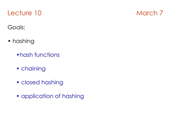
Lecture 10 March 7 Goals: hashing hash functions chaining closed hashing application of hashing. Computing hash function for a string Horner’s rule: (( … (a 0 x + a 1 ) x + a 2 ) x + … + a n-2 )x + a n-1 )

E N D
Lecture 10 March 7 • Goals: • hashing • hash functions • chaining • closed hashing • application of hashing
Computing hash function for a string Horner’s rule: (( … (a0 x + a1) x + a2) x + … + an-2 )x + an-1) int hash( const string & key ) { int hashVal = 0; for( int i = 0; i < key.length( ); i++ ) hashVal = 37 * hashVal + key[ i ]; return hashVal; }
Computing hash function for a string int myhash( const HashedObj & x ) const { int hashVal = hash( x ); hashVal %= theLists.size( ); return hashVal; } Alternatively, we can apply % theLists.size() after each iteration of the loop in hash function. int myHash( const string & key ) { int hashVal = 0; int s = theLists.size(); for( int i = 0; i < key.length( ); i++ ) hashVal = (37 * hashVal + key[ i ]) % s; return hashVal % s; }
Analysis of open hashing/chaining Open hashing uses more memory than open addressing (because of pointers), but is generally more efficient in terms of time. If the keys arriving are random and the hash function is good, keys will be nicely distributed to different buckets and so each list will be roughly the same size. Let n = the number of keys present in the hash table. m = the number of buckets (lists) in the hash table. If there are n elements in set, then each bucket will have roughly n/m If we can estimate n and choose m to be ~ n, then the average bucket will be 1. (Most buckets will have a small number of items).
Analysis continued Average time per dictionary operation: m buckets, n elements in dictionary average n/m elements per bucket n/m = l is called the load factor. insert, search, remove operation take O(1+n/m) = O(1+l) time each (1 for the hash function computation) If we can choose m ~ n, constant time per operation on average. (Assuming each element is likely to be hashed to any bucket, running time constant, independent of n.)
Closed Hashing Associated with closed hashing is a rehash strategy: “If we try to place x in bucket h(x) and find it occupied, find alternative location h1(x), h2(x), etc. Try each in order, if none empty table is full,” h(x) is called home bucket Simplest rehash strategy is called linear hashing hi(x) = (h(x) + i) % D In general, our collision resolution strategy is to generate a sequence of hash table slots (probe sequence) that can hold the record; test each slot until find empty one (probing)
Closed Hashing (open addressing) Example: m =8, keys a,b,c,d have hash values h(a)=3, h(b)=0, h(c)=4, h(d)=3 Where do we insert d? 3 already filled Probe sequence using linear hashing: h1(d) = (h(d)+1)%8 = 4%8 = 4 h2(d) = (h(d)+2)%8 = 5%8 = 5* h3(d) = (h(d)+3)%8 = 6%8 = 6 Etc. Wraps around the beginning of the table b 0 1 2 3 a c 4 d 5 6 7
Operations Using Linear Hashing • Test for membership: search • Examine h(k), h1(k), h2(k), …, until we find k or an empty bucket or home bucket case 1: successful search -> return true case 2: unsuccessful search -> false case 3: unsuccessful search and table is full • If deletions are not allowed, strategy works! • What if deletions?
Operations Using Linear Hashing • What if deletions? If we reach empty bucket, cannot be sure that k is not somewhere else and empty bucket was occupied when k was inserted • Need special placeholder deleted, to distinguish bucket that was never used from one that once held a value
Implementation of closed hashing Code slightly modified from the text. // CONSTRUCTION: an approximate initial size or default of 101 // // ******************PUBLIC OPERATIONS********************* // bool insert( x ) --> Insert x // bool remove( x ) --> Remove x // bool contains( x ) --> Return true if x is present // void makeEmpty( ) --> Remove all items // int hash( string str ) --> Global method to hash strings The same hash function can used in closed hashing and open hashing.
template <typename HashedObj> class HashTable { public: HashTable(int size) { theLists.resize( nextPrime(size)); makeEmpty(); } bool contains( const HashedObj & x ) const { return isActive( findPos( x ) ); } void makeEmpty( ) { currentSize = 0; for( int i = 0; i < array.size( ); i++ ) array[ i ].info = EMPTY; }
bool insert( const HashedObj & x ) { int currentPos = findPos( x ); if( isActive( currentPos ) ) return false; array[ currentPos ] = HashEntry( x, ACTIVE ); if( ++currentSize > array.size( ) / 2 ) rehash( ); // rehash when load factor exceeds 0.5 return true; } bool remove( const HashedObj & x ) { int currentPos = findPos( x ); if( !isActive( currentPos ) ) return false; array[ currentPos ].info = DELETED; return true; } enum EntryType { ACTIVE, EMPTY, DELETED };
private: struct HashEntry { HashedObj element; EntryType info; }; vector<HashEntry> array; int currentSize; bool isActive( int currentPos ) const { return array[ currentPos ].info == ACTIVE; }
int findPos( const HashedObj & x ) { int offset = 1; // int offset = s_hash(x); /* double hashing */ int currentPos = myhash( x ); while( array[ currentPos ].info != EMPTY && array[ currentPos ].element != x ) { currentPos += offset; // Compute ith probe // offset += 2 /* quadratic probing */ if( currentPos >= array.size( ) ) currentPos -= array.size( ); } return currentPos; }
Performance Analysis - Worst Case • Initialization: O(m), m = # of buckets • Insert and search: O(n), n number of elements currently in the table • Suppose there are close to n elements in the table that form a chain. Now want to search x, and say x is not in the table. It may happen that h(x) = start address of a very long chain. Then, it will take O(c) time to conclude failure. c ~ n. • No better than linear list for maintaining dictionary! • THIS IS NOT A RARE OCCURRENCE WHEN THE TABLE IS NEARLY FULL. (this is why we rehash when a reaches some value like 0.5)
Example II insert 1052 (h.b. 7) I 0 1001 0 1001 1 9537 1. What if next element has home bucket 0? go to bucket 3 Same for elements with home bucket 1 or 2! Only a record with home position 3 will stay. p = 4/11 that next record will go to bucket 3 1 9537 h(k) = k%11 = 0 2 3016 2 3016 3 3 4 4 5 5 6 6 7 9874 7 9874 8 2009 2. Similarly, records hashing to 7,8,9 will end up in 10 3. Only records hashing to 4 will end up in 4 (p=1/11); same for 5 and 6 8 2009 9 9875 9 9875 10 1052 10 next element in bucket 3 with p = 8/11
Performance Analysis - Average Case • Distinguish between successful and unsuccessful searches • Delete = successful search for record to be deleted • Insert = unsuccessful search along its probe sequence • Expected cost of hashing is a function of how full the table is: load factor l = n/m
Random probing model vs. linear probing model • It can be shown that average costs under linear hashing (probing) are: • Insertion: 1/2(1 + 1/(1 - l)2) • Deletion: 1/2(1 + 1/(1 - l)) • Random probing: Suppose we use the following approach: we create a sequence of hash functions h, h,… all of which are independent of each other. • insertion: 1/(1 – l ) • deletion: 1/l log(1/ (1 – l))
Random probing – analysis of insertion (unsuccessful search) What is the expected number of times one should roll a die before getting 4? Answer: 6 (probability of success = 1/6.) More generally, if the probability of success = p, expected number of times you repeat until you succeed is 1/p. If the current load factor = l, then the probability of success = 1 – l since the proportion of empty slots is 1 – l.
Improved Collision Resolution • Linear probing: hi(x) = (h(x) + i) % D • all buckets in table will be candidates for inserting a new record before the probe sequence returns to home position • clustering of records, leads to long probing sequence • Linear probing with increment c > 1: hi(x) = (h(x) + ic) % D • c constant other than 1 • records with adjacent home buckets will not follow same probe sequence • Double hashing: hi(x) = (h(x) + i g(x)) % D • G is another hash function that is used as the increment amount. • Avoids clustering problems associated with linear probing.
Comparison with Closed Hashing • Worst case performance is O(n) for both. Average case is a small constant in both cases when a is small. • Closed hashing – uses less space. • Open hashing – behavior is not sensitive to load factor. Also no need to resize the table since memory is dynamically allocated.