Download
1 / 21
210 likes | 370 Views
Static Dictionaries. Collection of items. Each item is a pair. (key, element) Pairs have different keys. Operations are: initialize/create get (search). Hashing. Perfect hashing (no collisions). Minimal perfect hashing (space = n ). CHD algorithm.

E N D
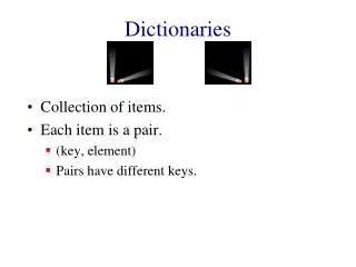
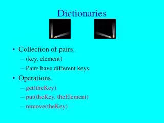
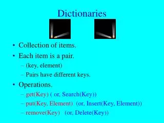
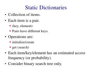
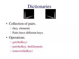
Static Dictionaries • Collection of items. • Each item is a pair. • (key, element) • Pairs have different keys. • Operations are: • initialize/create • get (search)
Hashing • Perfect hashing (no collisions). • Minimal perfect hashing (space = n). • CHD algorithm. • O(n) time to construct the perfect or minimal perfect hash function. • O(1) search time. • Bothelo, Belazzougui & Dietzfelbinger. Compress, hash, and displace. 17th European Symposium on Algorithms, 2009.
Search Tree • Hashing not efficient for extended operations such as range search and nearest match. • Will examine a binary search tree structure for static dictionaries. • Each item/key/element has an estimated access frequency (or probability).
a b b c a c Example a < b < c Cost = 0.8 * 1 + 0.1 * 2 + 0.1 * 3 = 1.2 Cost = 0.8 * 2 + 0.1 * 1 + 0.1 * 2 = 1.9
f0 f1 f2 f3 b c a Search Types • Successful. • Search for a key that is in the dictionary. • Terminates at an internal node. • Unsuccessful. • Search for a key that is not in the dictionary. • Terminates at an external/failure node.
f0 f1 f2 f3 b c a Internal And External Nodes • A binary tree with n internal nodes has n + 1 external nodes. • Let s1, s2, …, sn be the internal nodes, in inorder. • key(s1) < key(s2) < … < key(sn). • Let key(s0) = –infinity and key(sn+1) = infinity. • Let f0, f1, …, fn be the external nodes, in inorder. • fi is reached iff key(si)< search key <key(si+1).
f0 f1 f2 f3 b c a Cost Of Binary Search Tree • Let pi = probability for key(si). • Let qi = probability for key(si)< search key <key(si+1). • Sum of ps and qs = 1. • Cost of tree = S0 <= i <= n qi (level(fi) – 1) + S1<= i <= n pi *level(si) • Cost = weighted path length.
Brute Force Algorithm • Generate all binary search trees with n internal nodes. • Compute the weighted path length of each. • Determine tree with minimum weighted path length. • Number of trees to examine is O(4n/n1.5). • Brute force approach is impractical for large n.
a5 a6 a3 a7 a4 f5 f2 f7 f6 f4 f3 Dynamic Programming • Keys are a1< a2 < …<an. • Let Ti j= least cost tree for ai+1, ai+2, …, aj. • T0n= least cost tree for a1, a2, …, an. T2,7 • Ti j includes pi+1, pi+2, …, pj and qi, qi+1, …, qj.
a5 a6 a3 a7 a4 f5 f2 f7 f6 f4 f3 Terminology T2,7 • Ti j= least cost tree for ai+1, ai+2, …, aj. • ci j= cost of Ti j =Si <= u <= j qu (level(fu) – 1) + Si < u <= j pu *level(su). • ri j= root of Ti j. • wi j= weight of Ti j = sum of ps and qs in Ti j = pi+1+ pi+2+ …+ pj + qi + qi+1 + … + qj
Tii fi i = j • Ti j includes pi+1, pi+2, …, pj and qi, qi+1, …, qj. • Ti i includes qi only. • ci i = cost of Ti i = 0. • ri i = root of Ti i = 0. • wi i = weight of Ti i • = sum of ps and qs in Ti i • = qi
a5 ak a6 a3 Ti j a7 L R a4 f5 f2 f7 f6 f4 f3 i < j • Ti j= least cost tree for ai+1, ai+2, …, aj. • Ti j includes pi+1, pi+2, …, pj and qi, qi+1, …, qj. • Let ak, i < k <= j, be in the root of Ti j. • L includes pi+1, pi+2, …, pk-1 and qi, qi+1, …, qk-1. • R includes pk+1, pk+2, …, pj and qk, qk+1, …, qj.
a5 a6 a3 a7 L a4 f5 f2 f7 f6 f4 f3 cost(L) • L includes pi+1, pi+2, …, pk-1 and qi, qi+1, …, qk-1. • cost(L) = weighted path length ofL when viewed as a stand alone binary search tree.
ak Ti j L L R Contribution To cij • ci j =Si <= u <= j qu (level(fu) – 1) + Si < u <= j pu *level(su). • When L is viewed as a subtree of Ti j , the level of each node is 1 more than when L is viewed as a stand alone tree. • So, contribution of L to cij is cost(L) + wi k-1.
a5 ak a6 a3 Ti j a7 L R a4 f5 f2 f7 f6 f4 f3 cij • Contribution of L to cij is cost(L) + wi k-1. • Contribution of R to cij is cost(R) + wkj. • cij = cost(L) + wi k-1 +cost(R) + wkj + pk = cost(L) + cost(R) + wij
a5 ak a6 a3 Ti j a7 L R a4 f5 f2 f7 f6 f4 f3 cij • cij = cost(L) + cost(R) + wij • cost(L) = cik-1 • cost(R) = ckj • cij = cik-1 + ckj + wij • Don’tknow k. • cij = mini < k <= j{cik-1 + ckj}+ wij
ak Ti j L R cij • cij = mini < k <= j{cik-1 + ckj}+ wij • rij = k that minimizes right side.
Computation Of c0n Andr0n • Start with ci i =0, ri i =0, wi i =qi, 0 <= i <= n (zero-key trees). • Use cij = mini < k <= j{cik-1 + ckj}+ wij to compute cii+1, ri i+1, 0 <= i <= n – 1 (one-key trees). • Now use the equation to compute cii+2, ri i+2, 0 <= i <= n – 2 (two-key trees). • Now use the equation to compute cii+3, ri i+3, 0 <= i <= n – 3 (three-key trees). • Continue until c0n andr0n(n-key tree) have been computed.
1 2 3 4 0 0 1 2 3 4 cij, rij, i <= j Computation Of c0n Andr0n
Complexity • cij = mini < k <= j{cik-1 + ckj}+ wij • O(n) time to compute one cij. • O(n2)cijs to compute. • Total time is O(n3). • May be reduced to O(n2) by using cij = min ri,j-1 < k <= ri+1,j{cik-1 + ckj}+ wij
T0n a10 T09 T10,n Construct T0n • Root is r0n. • Suppose that r0n = 10. • Construct T09 and T10,n recursively. • Time is O(n).