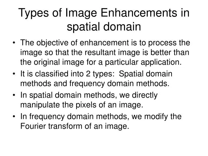
Types of Image Enhancements in spatial domain

1. Types of Image Enhancements in spatial domain • The objective of enhancement is to process the image so that the resultant image is better than the original image for a particular application. • It is classified into 2 types: Spatial domain methods and frequency domain methods. • In spatial domain methods, we directly manipulate the pixels of an image. • In frequency domain methods, we modify the Fourier transform of an image.

2. Spatial Domain • Spatial domain refers to the aggregate of pixels composing an image. It is expressed as: • g(x,y) = T[f(x,y)] • where f(x,y) is the input image, g(x,y) is the processed image and T is an operator on f, defined over some neighborhood of (x,y). • When we say neighborhood about a point (x,y) means use a square or rectangular subimage area centered at (x,y) as shown in figure.

3. A 3 x 3 neighborhood about a point (x, y) in an image

4. Gray Level Transformation • The centre of this subimage is moved from pixel to pixel starting from top left corner. • The operator T is applied at each location (x,y) to get the output, g, at that location. • For neighborhood, shapes such as circle are used. • But square and rectangular arrays are very common. When T is a 1 X 1 neighborhood, g depends only on the value of f at (x,y), and T becomes a gray-level (called intensity or mapping) transformation function of the form: • s = T(r) • Here r and s are variables denoting the gray level of f(x,y) and g(x,y) at any point (x,y).

5. Contrast Stretching • The effect of this transformation is to produce an image of higher contrast than the original by darkening the levels below m and brightening the levels above m in the original image. • This is called as contrast stretching. • Here the values of r below m are compressed by the transformation function into a narrow range of s, toward black. • For values of r above m, the opposite happens. • This produces a 2 level image called binary image. • A mapping of this form is called a thresholding function. • Here the enhnaement at any point in an image depends only on the gray level at that point, we call it as point processing.

8. Gray level transformation function for contrast enhancement

9. Mask Processing • One can also use larger neighborhoods called masks. • It is also called as filters, kernels, templates or windows. • Mask is a small (say, 3 X 3) 2-D array, in which the values of the mask coefficients determine the nature of the process such as image sharpening. • Enhancement techniques based on masks are called as mask processing or filtering.

10. Additive Image Offset • An additive Image offset has the form • g(x,y) = f(x,y) + L • Here L is an integer. • We assume that image is quantized into integers in the range {0,1,…,K-1}. I • f L >0, then g(x,y) will be a brightened image. • If L <0, then g(x,y) will be a dimmed image. • If |g(x,y)| becomes < 0 due to additive image offset operation, then we set |g(x,y)| = 0. • Similarly if |g(x,y)| > K-1, then we set |g(x,y)| = K-1. • This operation only improves the overall visibility of the image but it will not improve the contrast.

11. F = F+L(0.3) F = F-L(0.3)

12. clear all; close all; clc; f = imread('bird.gif'); f = im2double(f); figure,imshow(f),title('Gray Scale Image'); L = 0.3; f1 = f+L; figure,imshow(f1),title(‘Additive image '); f2 = f-L; figure,imshow(f2),title(‘Additive image');

13. Multiplicative Image Scaling • A multiplicative image scaling by a factor P is given by: • g(x,y) = Pf(x,y) • Here P is assumed to be positive as g(x,y) must be positive. • But P need not be an integer. • The practical definition for the output is to round the result as13 • g(x,y) = INT[Pf(x,y) + 0.5]. • If P > 1, then the gray levels of g will cover a broader range than those of f. • If P < 1, then g will have a narrower gray-level distribution than f. • Thus multiplicative scaling either stretches or compresses the image.

14. P=2 F1 = P*F P=0.5 F1 = P*F

15. clear all; close all; clc; f = imread('bird.gif'); f = im2double(f); figure,imshow(f),title('Gray Scale Image'); L = 2; f1 = f.*L; figure,imshow(f1),title('Multiplicativeimage'); L1 = 0.5; f2 = f.*L1; figure,imshow(f2),title('Multiplicative image');

16. Image Negative • The linear point operation that uses both scaling and offset is called the image negative and it is given by P = -1 and L = K-1. Hence • g(x,y) = -f(x,y) + (K-1) • The scaling by P = -1 reverses (flips) the histogram. • The additive offset L = K-1 is needed so that all values of the result are positive and fall in the allowable gray-scale range. • This operation creates a digital negative image. • If the image is already a negative, then it produces a positive image.

17. Negative of an image

18. % Read a gray scale image and generate the negative of it • % Read the negative image and by taking its negative get the original image • % Extend the same technique for color image • clear all; close all; clc; • a=imread('Cameraman.tif'); • b=im2double(a); • [m n]=size(b); • for i=1:m • for j=1:n • c(i,j)= 1-b(i,j); • end • end • figure,imshow(a); • figure,imshow(c);

19. Nonlinear Transformations • Log Transformations • The general form of log transformation is: • s = c log( 1 + r) • Here c is a constant and r ≥ 0. • The shape of the log curve implies that this transformation maps a narrow range of low gray-level values in the input image into a wider range of output levels. • The opposite is true for higher values of input levels. • This transformation can be used to expand the values of dark pixels in an image while compressing the higher level values. • The opposite is true of the inverse log transformation. Log transformations are mainly used in Fourier spectrum.

20. Fourier spectrum and Result of applying the log transformation

22. Power Law Transformations • This transformation has the form: • Here c and γ are positive constants. Like log transformations, power law curves with fractional values of γ map a narrow range of dark input values into a wider range of output values. • A variety of devices used for image capture, printing and display respond according to a power law. (eg) Cathode Ray Tube devices have an intensity-to-voltage response that is a power function, with exponents varying from 1.8 to 2.5. • The display systems tend to produce image that are darker than intended. • This transformation is also useful for contrast manipulation.

23. Power law transforms for various gamma values

24. Gamma = 0.2

25. Power-Law Transformations • % Read a gray scale image and apply the power-law transform for gamma • % =0.05,0.2,0.67,1.5,2.5,5 and comment your results • clear all; • close all; clc; • f = imread('pout.tif'); • f = im2double(f); • [m n]=size(f); • c = 1; • y=input('Gamma value:'); • for i=1:m • for j=1:n • s(i,j)=c*(f(i,j)^y); • end • end • figure,imshow(f); • figure,imshow(s);

26. Contrast stretching • Here low-contrast images can result from poor illumination, lack of dynamic range in the imaging sensor, or wrong setting of lens aperture during image acquisition. • The idea of contrast stretching is to increase the dynamic range of gray levels in the image. • Let us consider a transformation function used for contrast stretching. • If r1 = s1 and r2 = s2, the transformation is a linear function that produces no changes in gray levels. • If r1 = r2, s1 =0 and s2 = L-1, the transformation becomes a thresholding function that creates a binary image.

27. Contrast stretching

28. Contrast Stretching • clear all; close all; clc; • f = imread('cameraman.tif'); • f = im2double(f); • m=0.75; %contrast • E=0.55; %slope of the function • g = 1./(1+(m./(f+eps)).^E); • figure,imshow(f); • figure,imshow(g);

29. Gray level slicing • Highlighting a specific range of gray levels in an image is often useful. • To achieve this there are 2 approaches. • One approach is to display a high value for all gray levels in the range of interest and a low value for all other gray levels. • This also produces a binary image. • The other kind of transformation is used to brighten the desired range of gray levels but preserves background and gray-level tonalities in the image

30. Gray level slicing

31. Gray level slicing

32. % Gray scale slicing clear all; close all; clc; f = imread('cameraman.tif'); a = 100; b = 200; T1 = 25; T2 = 250; [m n]=size(f); for i=1:m for j=1:n if (f(i,j)< a || f(i,j) > b) f1(i,j)= T1; else f1(i,j)=T2; end end end

33. f1 = uint8(f1); figure,imshow(f); figure,imshow(f1); T3= 200; for i=1:m for j=1:n if (f(i,j) > a && f(i,j) < b) f2(i,j)= T3; else f2(i,j)=f(i,j); end end end f2 = uint8(f2); figure,imshow(f); figure,imshow(f2);

34. Bit plane slicing • Sometimes instead of highlighting the gray-level ranges, highlighting the contribution made to total image by specific bits is desirable. • Imagine that the image is composed of eight 1-bit planes, ranging from bit-plane 0 for the least significant bit to bit plane 7 for the most significant bit. • The plane 0 contains all lowest order or bits and plane 7 contains all the high order bits. • The higher order bits contain the majority of the visually significant data. • Other planes contain only subtle details. • This process can aid in determining the number of bits needed to quantize each pixel.

35. Bit plane slicing • To get the bit plane 7 one can threshold the image with a thresholding gray-level transformation function that maps all levels in the image between 0 and 127 (eg 0). • Map the levels between 129 and 255 to another (eg 255). • Similarly we can obtain the gray-level transformation function for other bit planes.

38. % bit plane slicing clear all; close all; clc; f = imread('onion.png'); f = rgb2gray(f); [m n] = size(f); f1(1:m,1:n)=0; s = input('Enter bit levels:'); b = [128,64,32,16,8,4,2,1]; b1 = [255,128,64,32,16,8,4,2,1]; for i = 1:m for j = 1:n for k=1:s if f(i,j)> b(k) f1(i,j)=f1(i,j)+b1(k); % break; else f1(i,j)=f1(i,j); end end end end f1=uint8(f1); figure,imshow(f); figure,imshow(f1);