Dynamic Product Assembly and Inventory Control for Maximum Profit

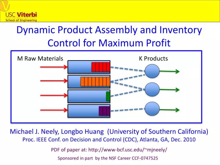
1. Dynamic Product Assembly and Inventory Control for Maximum Profit M Raw Materials K Products Michael J. Neely, Longbo Huang (University of Southern California) Proc. IEEE Conf. on Decision and Control (CDC), Atlanta, GA, Dec. 2010 PDF of paper at: http://www-bcf.usc.edu/~mjneely/ Sponsored in part by the NSF Career CCF-0747525

2. Product Assembly System M Raw Materials K Products Example Recipe for Product 1: [One unit of Product 1] = + Challenge: The “underflow” problem!

3. Product Assembly System M Raw Materials K Products A1(t) A2(t) A3(t) A4(t) • Raw Material Purchasing Decisions: • xm(t) = Randomcostfor material m on slot t. • Am(t) = Amount of material m we purchase on slot t. • Decision constraint: 0 ≤ Am(t) ≤ Ammax. Expense(t) = ∑mAm(t)xm(t)

4. Product Assembly System M Raw Materials K Products A1(t) P1(t) A2(t) P2(t) A3(t) P3(t) A4(t) • Product Pricing Decisions: • pk(t) = Price for product k chosen on slot t. • y(t) = Demand state for slot t. • Dk(t) = Random demand for product k on slot t. • Fk(p, y) = Demand Function = E{Dk(t)|pk(t)=p, y(t)=y}. Revenue(t) = ∑kpk(t)Dk(t) – Assembly Cost

5. About the Demand Function F() • Example 1: • Demand State y(t) in {High, Medium, Low, Zero}. • Fk(p, y) = E{Dk(t)|pk(t) = p, y(t) = y}. High Medium Expected demand Fk(p,y) Low price pk (for product k)

6. About the Demand Function F() • Example 2: • Special case of no pricing decisions. • pk(t) = pk (fixed at some constant for all time). • Y(t) = (Y1(t), …, YK(t)) = Random demand for slot t. • Dk(t) = Yk(t). M Raw Materials K Products A1(t) D1(t) A2(t) D2(t) A3(t) D3(t) A4(t)

7. Problem Formulation: • Every slot t, observe: • Queue states Qm(t) • Raw material prices pm(t) • Demand state y(t). • Make purchasing decisions (Am(t)) and pricing • decisions (pm(t)) to maximize time average profit: • Average Profit = limtinfinity (1/t)∑τ=0 Profit(τ) • Profit(t) = Revenue(t) – Expense(t) t-1

8. Solution Strategy: Dynamic Queue Control θm Qm(t) • Want to keep queue size high to avoid underflow. • Don’t want queues too high (un-used inventory). • Lyapunov Function (same as the stock market work): • L(Q(t)) = ∑m(Qm(t) – θm)2

9. Control Design: Qn(t) • Lyapunov Function L(Q(t)) • Lyapunov Drift Δ(t) = L(Q(t+1)) – L(Q(t)) • Every slot t, observe Q(t), p(t), and • minimize the drift-plus-penalty*: θn Δ(t) - V xProfit(t) *from stochastic network optimization theory [Georgiadis, Neely, Tassiulas 2006][Neely 2010] Results in the following algorithm: • (Raw Material Purchasing) Observe costs (xm(t)). • Am(t) = Ammax, if Vxm(t) + Qm(t) ≤ θm • Am(t) = 0 , if Vxm(t) + Qm(t) > θm

10. Control Design: Qn(t) • Lyapunov Function L(Q(t)) • Lyapunov Drift Δ(t) = L(Q(t+1)) – L(Q(t)) • Every slot t, observe Q(t), p(t), and • minimize the drift-plus-penalty*: θn Δ(t) - V xProfit(t) *from stochastic network optimization theory [Georgiadis, Neely, Tassiulas 2006][Neely 2010] Results in the following algorithm: • (Product Pricing) Observe demand state y(t). • Max: Vpk(t)Fk(pk(t), y(t)) + Fk(pk(t),Y(t))∑mβmk(Qm(t) – θm) • Subject to: 0 ≤ pk(t) ≤ pkmax ( βmk = Num type m materials used for product k. )

11. Theorem (iid case): Suppose random (xm(t), y(t)) Vector is iid over slots. *Choose θm= C1 + C2V. Then: For all slots t we have: μmmax ≤ Qm(t) ≤ θm + Ammax (and thus never have underflow) For all slots t>0 we have: (1/t) ∑τ=0E{Profit(τ)} ≥ Profitopt - B/V - L(Q(0))/(Vt) With prob 1 we have: t-1 limtinfinity (1/t)∑τ=0 Profit(τ) ≥ Profitopt – B/V *μmmax = Max departures of raw material m on one slot. *The constants C1, C2 depend on βmk, Pkmax, μmmax, Ammax, and are given in the paper.

12. Theorem (iid case): Suppose random (xm(t), y(t)) vector is iid over slots. *Choose θm= C1 + C2V. Then: For all slots t we have: μmmax ≤ Qm(t) ≤ θm + Ammax (and thus never have underflow) For all slots t>0 we have: (1/t) ∑τ=0E{Profit(τ)} ≥ Profitopt - B/V - L(Q(0))/(Vt) With prob 1 we have: t-1 limtinfinity (1/t)∑τ=0 Profit(τ) ≥ Profitopt – B/V Can also extend to the non-iid case via “universal scheduling” techniques.

13. Extensions for Multi-Hop and Recent Related Work: • Multi-Hop “Processing” or “Product Assembly” Networks are of recent interest and can be used as models for manufacturing,network coding, cloud computing,data fusion. • Using max-weight backpressure doesn’t work (underflow problems). • Multi-Hop “Processing Networks” and theDeficit-Max-Weight Algorithm asymptotically avoids underflows for networks with some limitations [Jiang, WalrandAllerton 2009] [Jiang, Walrand, Morgan&Claypool 2010]. • Recent work by [Huang, Neely, ArXiv 2010] uses the Lyapunov function L(Q(t)) = ∑m(Qm(t) – θm)2 to avoid underflows in multi-hop. Different intuition given by Huang interprets this Lyapunov function as “lifting” the Lagrange multipliers for equality constraints to ensure they are non-negative (corresponding to physical systems). This intuition can yield improved O(log2(V)) buffer size tradeoffs! Qn(t) θm

14. Conclusions: M Raw Materials K Products • Product Assembly System with “Recipe” for each • product. • Dynamic Purchasing and Pricing avoids underflows. • Gets O(V) worst-case queue backlog. • Gets within O(1/V) of optimal time average profit.