Download
1 / 45
490 likes | 792 Views
Inventory Control. Mahmut Ali GÖKÇE Industrial Systems Engineering Dept. İzmir University of Economics. Some Basic Definitions. An inventory is an accumulation of a commodity that will be used to satisfy some future demand. Inventories of the following form: - Raw material

E N D
Inventory Control Mahmut Ali GÖKÇE Industrial Systems Engineering Dept. İzmir University of Economics
Some Basic Definitions • An inventory is an accumulation of a commodity that will be used to satisfy some future demand. • Inventories of the following form: - Raw material - Components (subassemblies) - Work-in-process - Finished goods - Spare parts - Purchased products in retailing
Functional Classification of Inventories • Anticipation Stock: You have to keep some inventory to satisfy the expected demand of the customer. • Customer comes to the store and requires immediate purchase of what s/he needs. • You have to keep some items ready to satisfy such immediate requests based on your anticipation of the average demand • These inventories are referred to as anticipation stock
inventory cycle stock time a cycle Functional Classification of Inventories • Cycle Inventories: produce or buy in larger quantities than needed. • Economies of scale • Quantity discounts • Restrictions (technological,transportation,…)
inventory place order at this time time Safety stock reorder level Functional Classification of Inventories • Safety Stock: Provides protection against irregularities and uncertainties, in order to avoid stockouts.
Average Anticipation stock Low demand season Functional Classification of Inventories • Production Smoothing: Consider, low demand in one part of the year, hence build up stock for the high demand season.
Functional Classification of Inventories • Hedge inventories : expect changes in the conditions (price, strike, supply, etc.) • Pipeline (or work-in-process) inventories: goods in transit,between levels of a supply chain, between work stations.
Characteristics of Inventory Systems • Demand • Constant versus Variable • Known versus Random • Lead Time • Review Time • Periodic or Continuous • Excess Demand • Backorder allowed - Lost – Partial - Impatience • Changing Inventory • Perishable or Not
Framework for Inventory Control • Large number of items • Large manufacturer ~ 500,000 items • Retailer ~ 100,000 • Items show different characteristics • Demand can occur in many ways: • Unit by unit, in cases, by the dozen, etc.
Goals: Reduce Cost, Improve Service • By effectively managing inventory: • Xerox eliminated $700 million inventory from its supply chain • Wal-Mart became the largest retail company utilizing efficient inventory management • GM has reduced parts inventory and transportation costs by 26% annually
Goals: Reduce Cost, Improve Service • By not managing inventory successfully • In 1994, “IBM continues to struggle with shortages in their ThinkPad line” (WSJ, Oct 7, 1994) • In 1993, “Liz Claiborne said its unexpected earning decline is the consequence of higher than anticipated excess inventory” (WSJ, July 15, 1993) • In 1993, “Dell Computers predicts a loss; Stock plunges. Dell acknowledged that the company was sharply off in its forecast of demand, resulting in inventory write downs” (WSJ, August 1993)
Understanding Inventory • The inventory policy is affected by: • Demand Characteristics • Lead Time • Number of Products • Objectives • Service level • Minimize costs • Cost Structure
Cost Structure • Order costs • Fixed (Set-up cost, K) • Variable (c) • Holding Costs (h) • Insurance • Maintenance and Handling • Taxes • Opportunity Costs • Obsolescence (risk of loosing some of its value) • Stock out Cost (p) • Customer goodwill • Lost sales
3 Basic Questions Decision making in production and inventory management involves dealing with large number of items, with very diverse characteristics and with external factors. We want to resolve: • How often the inventory status (of an item) should be determined ? • When a replenishment order should be placed ? • How large the replenishment order should be ?
Why EOQ ? Economic Order Quantity • Easy to compute • Does not require data that is hard to obtain • Policies are surprisingly robust • Assumptions can be relaxed • Gives a good overall idea • Can be starting point for more complicated models
Assumptions Leading to EOQ • Demand rate, D, is constant and deterministic over time (units/day, units/year, etc.) • The order quantities are fixed at Q items per order, need not be discrete, and there are no minimum or maximum restrictions • Unit variable cost, v, does not depend on Q (no discounts) • A fixed cost K is incurred every time an order is placed • Cost factors do not change over time • Single item (no interaction with others)
EOQ Assumptions (Continued) • Replenishment lead time is negligible • No shortages are allowed • Entire order quantity is delivered at the same time • The planning horizon is infinite • The initial inventory is 0 As we will see, these assumptions can be relaxed.
Economic Order Quantity Model • Our aim is to determine the best replenishment strategy (recall: when and how much to order) under the criterion that the relevant costs will be minimized over time (i.e., minimize cost per unit time) • It is reasonable to consider the following optimization problem:
EOQ Model - Intuition • When we should place a new replenishment order ? • Demand is deterministic and at a constant rate • lead time is negligible • no backorders are allowed • Hence, a replenishment order should be placed each time inventory level drops to zero
EOQ Model - Intuition • How much we have to order each time ? • Parameters do not change over time ! • There is no reason for ordering different quantities. So, each time a replenishment order is placed we order the same quantity Q
EOQ - Notation Recall the notation we introduced earlier: Q = replenishment order quantity K = fixed cost incurred with each replenishment c = unit variable cost of an item $/unit h = the holding cost D = demand rate, units/unit time
Q -D Time Economic Lot Size Model • Costs: • K: order cost • h: inventory holding cost • Q : order size (decision var.) Inventory T
Deriving EOQ • Note from the figure that the same picture occurs over and over again (why ? Everything is stationary over time!) . Any one of the triangles will be called a “cycle”. Then,
Deriving EOQ • Cycle timeT =Q/D (slope, -D, = -Q/T) Since Q/D is the time between two replenishments (and the cycle time), D/Q is the number of replenishments per unit time (4 months between two replenishments will give 0.25 replenishments per month). In each replenishment we pay, K+Qc (at each cycle) Replenishment costs/unit time =
Deriving EOQ • In each replenishment cycle the total inventory carried is the area of one triangle. Why ? It can be computed as • Then inventory carried per unit time (average inventory) is Q/2 (also by intuition !). • Inventory holding cost/unit time = Q h /2 • Inventory holding cost at each cycle = Q hT /2
G(Q) Ordering Cost Holdingcost Totalcost G(Q) Q Q* EOQ: Total Cost is Convex
EOQ: Total Cost is Convex Let’s verify: For Q > 0 TRC(Q) is convex
Deriving EOQ • Average inventory level in a cycle is Q/2 • Average inventory cost at each cycle is hTQ/2 • Total cost at every cycle is C(Q)= K + hTQ/2 • Cycle timeT =Q/D • Cost per unit time is KD/Q + hQ/2
G(Q) Ordering Cost Holding cost Total cost G(Q) Q Q* EOQ: Costs
Turnover Ratio • Turnover Ratio: A measure of effective inventory control = D/(Average Inventory) = At optimal Q value
EOQ: An Example • Number 2 pencils at the bookstore are sold at a fairly steady rate of 60 per week. The pencils cost the book store 2 cents each and sell for 15 cents each. It costs the book store $12 to initiate an order, and holding costs are based on an annual interest rate of 25%. Determine the optimum number of pencils for the bookstore to purchase and the time between placements of orders. What are the yearly holding and setup costs for the item?
EOQ: An Example • h= I*c=0.25*0.02=0.005 $ per unit per year • Order Quantity that Minimizes Average Total Cost = (2KD/h)1/2 = (2*12*3120/.005)1/2 = 3870 units T: cycle time = Q/D=3870/3120 = 1.24 years Average annual holding cost = hQ/2=.005*3870/2=$9.675 Average Annual setup cost = KD/Q = 12*3120/3870=$9.675
Inventory Q s=LD Time L Order given Order Arrives EOQ: lead time
EOQ: Sensitivity • If we cannot order Q units? G(Q) = KD/Q + hQ/2 G(Q*) = KD/ Q* + h Q*/2 = = For any other Q
EOQ: Sensitivity • Let Q*=3870. What if we order Q=1000 • G(Q) /G(Q*) = 0.5 (3.87 +1/3.87) = 2.06 • We can conclude that G(Q) is relatively insensitive to errors in Q • Hence one can order 4000 pencils if space available rather than 3870!
I H -D P-D Time T1 T2 T Relaxing EOQ: Production
EOQ:Production - Example • A local company produces programmable EPROM for several industrial clients. It has experienced a relatively flat demand of 2,500 units per year for the product. The EPROM is produced at a rate of 10,000 units per year. The accounting department has estimated that it costs $50 to initiate a production run, each unit costs the company $2 to manufacture, and the cost of holding is based on a 30 percent annual interest rate. Determine the optimal size of a production run, the length of each production run, and the average cost of holding and setup. What is the maximum level of on-hand inventory of EPROMs? (Nahmias, p. 213)
Relaxing EOQ: Quantity Discounts G(Q) G0(Q) G1(Q) G2(Q) Q 500 1000
Multiproduct Systems: A-B-C Analysis • There is a trade off between the cost of controlling the system and the potential benefits from that control. • Vilfredo Pareto studied the distribution of wealth in 19th century and noted that large portion of the wealth is owned by small segment of the population. • Typically the top 20% of the items account for the 80% of the annual dollar value of sales, the next 30 percent for the next 15. • To use ABC: • select criterion for ranking • rank items on basis of criterion • calculate percentages • set up classes around break points
Example A-B-C Analysis: Cumulatives 5 24.22064 (=39340/162426) 10 45.02026 15 62.86979 20 79.98034 25 89.1277 30 92.82754 35 96.23547 40 99.04374 45 99.46436 50 99.65564 55 99.73275 60 99.80628 65 99.86058 70 99.91023 75 99.94351 80 99.96693 85 99.98471 90 99.99231 95 99.9982 100 100
A-B-C Analysis • Since A items account for the lion’s share of the yearly revenue, these items should be watched closely and inventory levels for A items should be the monitored continuously. • More sophisticated forecasting techniques might be used • More care would be taken in the estimation of the various cost parameters required in calculating optimal policies.