Download
1 / 62
730 likes | 1.39k Views
Theories of Classical Conditioning. Critical CS-US relationship. Important (critical) things to note about classical conditioning: the CS MUST precede the US the CS MUST predict the US if the CS does not predict the US, no conditioning occurs

E N D
Critical CS-US relationship • Important (critical) things to note about classical conditioning: • the CS MUST precedethe US • the CS MUST predict the US • if the CS does not predict the US, no conditioning occurs • the CR does not have to be identical to the UR • E.g., subtle differences even Pavlov noticed) • may even be opposite: Morphine studies • Any response is a classically conditioned response if it • Occurs to a CS • After that CS has been paired with a US • But does NOT occur to a randomly presented CS-US pairing
Theories of Classical Conditioning: WHY do organisms respond to predictability? • Pavlov: Stimulus substitutability theory and Perceptual Gating Theory • Kamin: Surprise theory • Rescorla and Wagner: Computational Model • Current Attentional Models
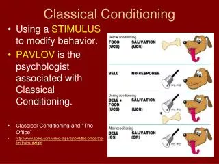
Pavlov: Stimulus Substitution Theory • Basic premise of SST theory: CS substitutes for US • With repeated pairings between CS and US, CS becomes substitute for the US • Thus, the response initially elicited only by US is now also elicited by CS • Sounds pretty good: • Salivary conditioning: US and CS both elicit salivation • Eyeblink conditioning: both elicit eyeblinks • Theory was doing well until we found compensatory CRs
Pavlov: Stimulus Substitution Theory • Criticisms and Flaws: • CR is almost never an exact replica of the UR • An eyeblink to UR of air puff = large, rapid closure • Eyeblink to CS of tone = smaller, more gradual closure • Defense of theory: Hilgard (1936): Why differences in CR and UR: • Intensity and stimulus modality of the CS and US are different • Thus: differences in Response magnitude and timing are to be expected • But still doesn’t explain OPPOSITE CR
Pavlov: Stimulus Substitution Theory • BIGGER PROBLEM: • Whereas many USs elicit several different Rs, as a general rule not all of these Rs are later elicited by the CS • CS seems to select for certain CRs • E.g. Zener (1937) • Dog presented w/food as US: • Found that the dog elicited a number of UR responses to the food • E.g., salivation, chewing, swallowing, etc. • CS not elicit all of those responses • NO CRs of chewing and swallowing • Just the CR of just salivation • On other hand: CR may contain some responses that are not part of CR: • Zener found that dogs turned head to bell • But no head turns to presentation of food
Modifications of SST • MODIFICATIONS OF SST: (Hilgard) • Only some components of UR transferred to CR • CS such as a bell often elicits unconditioned responses of its own, and these may become part of CR • Remember SIGN TRACKING: Brown and Jenkins 1974 • Emphasized this change in form of CR vs. UR • Also Jenkins, Barrara, Ireland and Woodside (1976) • Sign Tracking : Animals tend to • Orient themselves toward the CS (not the US) • Approach • Explore any stimuli that are good predictors of important events such as the delivery of food
1 • Set up: • Initial training: Light turns on above feederfeeder releases pieces of hot dog • Test: • Light turns on above feeder, then above each of the other walls • Forms a sequence of 1234 • What is optimal response? • But: Dog “tracked the sign” 4 2 3 • Jenkins, Barrara, Ireland and Woodside (1976)
Modifications of SST • Strongest data against SST theory: Paradoxical conditioning • CR in opposite direction of UR • Black (1965): • Heart rate decreases to CS paired w/shock • US of shock elicits UR of heart rate INCREASE • But CS of light or tone elicits CR of heart rate DECREASE • Seigel (1979): Conditioned Compensatory Responses • Morphine studies • evidence of down regulation in addiction • Actual cellular process in neurons (and other cells, too!) • thus SST theory appears incorrect
Perceptual Gating Theory • Perceptual gating theory: • Idea that only if CS is biologically relevant will it get processed • If a CS doesn’t get processed it can be predictive/informative • Animals attend to biologically relevant stimuli • Problem: • Data show that under certain circumstances a stimulus is “attended to” or “processed”, but still does not serve as a CS with an accompanying CR • Issue remains: is the stimulus the most predictive? • Second issue: Defining “biologically relevant”
Kamin’s work: 1967-1974Blocking and overshadowing • Overshadowing: • Use one "weak" and one "strong" CS • E.g.: Bright light with soft tone • Train (CS1+CS2) US • Reaction to weaker stimulus is blotted out by stronger CS • Demonstrated by Pavlov
Kamin’s work: 1967-1974Blocking and overshadowing • CS(strong)+ CS (weak) US(shock) UR(avoidance) CR is STRONGEST CR (avoidance) • CS(strong) US(shock) UR(avoidance) CR is STRONG CR (avoidance • CS(weak) US(shock) UR(avoidance) CR is WEAK CR (avoidance
Kamin’s work: 1967-1974Blocking and overshadowing • Blocking: • Train 1 CS, then add a second CS to it: • CS1(light) US(shock)UR(avoidance) CR(avoidance) • CS1(light)+CS2(tone)US(shock) UR (avoidance) CR (avoidance) • Test each individually after training • CS1(light) US(shock)UR(avoidance) CR(avoidance) • CS2(tone) US(shock)UR(avoidance) CR(NO or very little avoidance) • Find that only one supports a CR • One stimulus “blocks” learning to second CS • Demonstrated by Kamin
Kamin’s blocking experiment • Used multiple CS's and 4 groups of rats • The blocking groupreceives • Series of L+ trials which produce strong CR • Series of L+T trials • Then tested to just the T • The Control groups receives SAME TOTAL NUMBER OF TRIALS AS BLOCKING GROUP • Group 1: No first phase; just test T • Group 2: L+ only; Test T • Group 3: T+ only; Test T • Group 4: LT+ only: Test T
Kamin’s blocking experiment • Prediction: Since both received same # of trials to the tone- should get equal conditioning to the tone • Results quite different: Blocking group shows no CR to the tone- the prior conditioning to the light "blocked" any more conditioning to the tone • Directly contradicts frequency principle (remember associationism!) Group Phase I Phase II Test Phase Result Control --- L+ T T elicits no CR Control --- T+ T T elicits CR Control --- LT+ T T elicits a CR Blocking L+ LT+ T T elicits no CR
Things we know about blocking: • The animal does "detect" the stimulus: • can’t be perceptual gating issue • EXT of CR with either T alone or with LT • EXT occurred faster with compound LT • Appears to be independent of: • length of presentation of the CS • number of trials of conditioning to compound CS • Constancy of US from phase 1 to 2 important!!!! • US must remain identical between the two phases or no blocking • Influenced by: • Type of CR measure (used CER, not as stable as non fear CR) • nature of CS may be important- e.g. modality • intensity of CS or US stimuli important • Depends on amount of conditioning to blocking stimulus which already occurred
Change in either US or CS can prevent/ overcome blocking • Change the intensity of the US from phase 1 to phase 2 • Change from 1 ma to 4 ma shock • L+ 1 ma shock • L+T 4 ma shock • Quickly condition to compound stimulus • Little or no overshadowing or blocking • Change in intensity of either CS stimulus- • Change in context from Phase 1 to Phase 2 • L(bright) shock • L(dim) T shock • Presents a different learning situation and no blocking: good response to both Light and Tone • Any ideas about what is happening?
Explanations of Blocking: • Poor Explanation: Perceptual gating theory: • tone never gets processed • tone not informative • data not really support this (evidence that do “hear” tone) • Good Explanation: Kamin's Surprise theory: • To condition requires some mental work on part of animal • Animal only does mental work when surprised • Bio genetic advantage: prevents having to carry around excess mental baggage • Thus only learn with "surprise" • Situation must be different from original learning situation • Better Explanation: Rescorla Wagner model: • particular US only supports a certain amount of conditioning • if one CS “hogs” all that conditioning- none is left over for another CS to be added • question- how do we show this?
A Brief Aside • Must determine how CS-US relationship works • Rescorla (1966) spent a lot of time on control groups • What exactly IS a control group in classical conditioning? • Why is this important? • Question of contiguity vs. predictability at play here.
Recorla: Which is more important?CS-US correlation vs. contiguity • CS-US contiguity: • CS and US are next to one another in time/space • In most cases, CS and US are continguous • CS-US correlation: CS followed by the US in a predictive correlation: • If perfect correlation (most predictive)- most conditioning • p(US/CS) = 1.0 • p(US/no CS) = 0.0 • But: life not always a perfect correlation
CS-US correlation is more critical • Rescorla (1966, 1968): Showed how 2 probabilities interact to determine size of the CS • CS = 2 min tone; presented at random intervals (M = 8 min) • Group 1: p(shock/CS) = 0.4correlation between CS and US during 2 min presentation • Group 2: p(shock/no CS) = 0.2 correlation between CS and US during 2 min presentation. • Which group should show more conditioning? • WHY?
Robert Rescorla (1966)Examined predictability 6 types of Groups • CS-alone: control group gets only the CS • Present CS alone with no US pairing • Problem: not have same number of US trials as experimental animals do, may actually be extinction effect • Novel CS group: present a novel CS to control group • Looks at whether stimulus is truly "neutral" • May produce habituation- animal doesn't respond because it "gets used to it" • US-alone: control group gets only the US • Present US alone with no CS pairing • Problem: not have same number of CS trials
Rescorla: 6 types of control groups • Explicitly unpaired control • CS NEVER predicts US • That is- presence of CS is really CS-, predicts NO US • Animal learns new rule: if CS, then no US • Backward conditioning: • US precedes CS • Assumes temporal order is important (but not able to explain why) • Again, animal learns that CS predicts no US, but US predicts CS • Discrimination conditioning (CS+ vs CS-) • Use one CS as a plus; one CS as a minus • Same problem as explicitly unpaired and backward • Works, but teaching a discrimination, not a control group
CS-US correlation: Summary of Results • Whenever p(US|CS) > p(US|NO cs): • CS = EXCITATORY CS • That is, CS predicts US • Amount of learning depended on size difference between p(US/CS) and p(US/no CS) • Whenever p(US|CS) <p(US|NO CS): • CS = INHIBITORY CS • CS predicts ABSENCE of US • Amount of learning depended on size difference between p(US/CS) and p(US/no CS) • Whenever p(US|CS) = p(US|NO CS): • CS = NEUTRAL CS • CS doesn’t predict or not predict CS • No learning will occur because there is no predictability.
CS-US correlation vs. contiguity • Thus: appears to be the CORRELATION between the CS and US, not the contiguity (closeness in time) that is important • Can write this more succinctly: • Correlation carries more information than contiguity • If R = + then excitatory CS • If R = - then inhibitory CS • If R = 0 then neutral CS (not really even a CS)
Classical condition is “cognitive”(oh the horror of that statement, I am in pain) • PREDICTABILITY is critical • Learning occurs slowly, trial by trial • Each time the CS predicts the US, the strength of the correlation is increased • The resulting learning curve is monotonically increasing: • Initial steep curve • Levels off as reaches asymptote • There is an asymptote to conditioning to the CS: • Maximum amount of learning that can occur • Maximum amount of responding that can occur to CS in anticipation of the upcoming US • We can explain this through an equation!
Rescorla Wagner Model Classical Conditioning and prediction
Theories of Classical Conditioning: WHY do organisms respond to predictability? • Ruled out • Pavlov: Stimulus substitutability theory • Perceptual Gating Theory • Kamin: Surprise theory: • Right, but wrong • Provided some really puzzling results • Rescorla and Wagner: Computational Model • Current Attentional Models
Kamin’s work: 1967-1974Blocking and overshadowing • Overshadowing: • Use one "weak" and one "strong" CS • CS1+CS2US • Reaction to weaker stimulus is blotted out by stronger CS • Demonstrated by Pavlov • CS(strong)+ CS (weak) US(shock) UR(avoidance) CR is STRONGEST CR (avoidance) • CS(strong) US(shock) UR(avoidance) CR is STRONG CR (avoidance • CS(strong) US(shock) UR(avoidance) CR is WEAK CR (avoidance
Kamin’s work: 1967-1974Blocking and overshadowing • Blocking: • Train 1 CS, then add a second CS to it: • CS1(light) US(shock)UR(avoidance) CR(avoidance) • CS1(light)+CS2(tone)US(shock) UR (avoidance) CR (avoidance) • Test each individually after training • CS1(light) US(shock)UR(avoidance) CR(avoidance) • CS2(tone) US(shock)UR(avoidance) CR(NO avoidance) • Find that only one supports a CR • One stimulus “blocks” learning to second CS • Demonstrated by Kamin
The Rescorla Wagner Equation!: • Yields an equation: THE Rescorla Wagner (1974) model!!!!! ΔV=k( λ-V0 or Vi =αißj(λj-Vsum) • Vi = amount learned (conditioned) on a given trial • Αi = the salience of the CS • ßj = the salience of the US • (λj-Vsum) = total amount of conditioning that can occur to a particular CS-US pairing
The Rescorla Wagner Equation!: • Yields an equation: THE Rescorla Wagner (1974) model!!!!! Vi =αißj(Λj-Vsum) • What does this equation say? • The amount of conditioning that will occur on a given trial is a function of: • The size of the salience of the CS multiplied by • The size of the salience of the US multiplied by • (The maximum amount of learning) - (the amount of learning that has already occurred).
Can say this easier! • How much you will learn on a given trial (Vi) is a function of: • αi or how good a stimulus the CS is (how well it grabs your attention) • ßjor how good a stimulus the US is (how well it grabs your attention • λj or how much can learning can be learned about the CS-US relationship • AND Vsum or how much you have learned ALREADY!
Assumptions of Rescorla-Wagner (1974) model • Model developed to accurately predict and map learning as it occurs trial by trial • Assumes a bunch of givens: • Assume animal can perceive CS and US, and can exhibit UR and CR • Helpful for the animal to know 2 things about conditioning: • what TYPE of event is coming • the SIZE of the upcoming event • Thus, classical conditioning is really learning about: • signals (CS's) which are PREDICTORS for • important events (US's)
Assumptions of R-W model • Assumes that with each CS-US pairing 1 of 3 things can happen: • The CS might become more INHIBITORY • The CS might become more EXCITATORY • There is no change in the CS • How do these 3 rules work? • If US is larger than expected: CS = excitatory • If US is smaller than expected: CS= inhibitory • If US = expectations: No change in CS • The effect of reinforcers or nonreinforcers on the change of associative strength depends upon: • The existing associative strength of THAT CS • AND on the associative strength of other stimuli concurrently present
More assumptions • Explanation of how an animal anticipates what type of CS is coming: • Direct link is assumed between "CS center" and "US center": • E.g. between a tone center and food center • In 1970’s: other researchers thought R and W were crazy with this idea • Now: neuroscience shows formation of neural circuits! • Assumes that STRENGTH of an event is given • The conditioning situation is predicted by the strength of the learned connection • THUS: when learning is complete: • The strength of the association relates directly to the size or intensity of the CS • Asymptote of learning = max learning that can occur to that size or intensity of a CS • Maximum amount of learning that a given CS can support
More assumptions • The change in associative strength of a CS as the result of any given trial can be predicted from the composite strength resulting from all stimuli presented on that trial: • Composite strength = summation of conditioning that occurs to all stimuli present during a conditioning trial • If composite strength is LOW: • the ability of reinforcer to produce increments in the strength of component stimuli is HIGH • More can be learned for this trial • If the composite strength is HIGH: • reinforcement is relatively less effective (LOW) • Less can be learned for this trial- approaching max of learning
More assumptions: • Can expand to extinction, or nonreinforcedtrials: • If composite associative strength of a stimulus compound is high, then the degree to which a nonreinforced presentation will produce a decrease in associative strength of the components is LARGE • If composite associative strength is low- nonreinforcement effects reduced
WHY is this equation important? • We can use the three rules to make predictions about amount and direction of classical conditioning • λ j > Vsum = Excitatory Conditioning • The degree to which the CS predicted the size of the US was GREATER than expected, so you react MORE to the CS next trial • λ j < Vsum = Inhibitory Conditioning • The degree to which the CS predicted the size of the US was LESS than expected, so you react LESS to the CS next trial • λ j = Vsum = no change: • The CS predicted the size of the US exactly as you expected
The Equation: Let’s USE it to Explain Learning, Overshadowing and Blocking!: Vi =αißj(Λj-Vsum) • Vi = amount learned (conditioned) on a given trial • Αi = the salience of the CS • ßj = the salience of the US • (λj-Vsum) = total amount of conditioning that can occur to a particular CS-US pairing
Okay, you got all that? Let’s put this baby to work…….. …….we will try a few examples
The equation: Vi =αißj(λ j-Vsum) • Vi= change in associative strength that occurs for any CS, i, on a single trial • αi = stimulus salience (assumes that different stimuli may acquire associative strength at different rates, despite equal reinforcement) • ßj= learning rate parameters associated with the US (assumes that different beta values may depend upon the particular US employed) • Vsum = associative strength of the sum of the CS's (strength of CS-US pairing) • λ j= associative strength that some CS, i, can support at asymptote • In English: How much you learn on a given trial is a function of the value of the stimulus x value of the reinforcer x (the absolute amount you can learn minus the amount you have already learned).
Acquisition • FIrst conditioning trial: Assume (our givens) • CS = light; US= 1 ma Shock • Vsum = Vl; no trials so Vl = 0 • Thus: λ j-Vsum = 100-0 = 100 • First trial must be EXCITATORY • BUT: must consider the salience of the light: • αi= 1.0 • ßj = 0.5
Acquisition • Plug into the equation: • for TRIAL 1 • VL1 = (1.0)(0.)(100-0) = 0.5(100) = 50 • thus: VL1 only approaches 50% of the discrepancy between λj and Vsum is learned for the first trial
Acquisition • TRIAL 2: • Same assumptions! • VL2 = (1.0)(0.5)(100-50) = 0.5(50) = 25 • Vsum= (50+25) = 75
Acquisition • TRIAL 3: • VL3 = (1.0)(0.5)(100-75) = 0.5(25) = 12.5 • Vsum = (50+25+12.5) = 87.5
Acquisition • TRIAL 4: • VL = (1.0)(0.5)(100-87.5) = 0.5(12.5) = 6.25 • Vsum = (50+25+12.5+6.25) = 93.75 • TRIAL 10:Vsum = 99.81, etc., until reach ~100 on approx. trial 14 • When will you reach asymptote?
Now: Back to ExplainingBlocking and Overshadowing • Overshadowing: • use one "weak" and one "strong" CS • reaction to weaker stimulus: less CR • Reaction to stronger stimulus: more CR • Blocking: 1st CS blocks learning to 2nd CS • At issue: What is predicting what? • Does LT give any more information/predictability than L alone? • If not, then L “blocks” learning to LT
How to explain overshadowing? Yep, it is good old Rescorla-Wagner to the rescue!