Download

1 / 27
280 likes | 447 Views
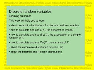
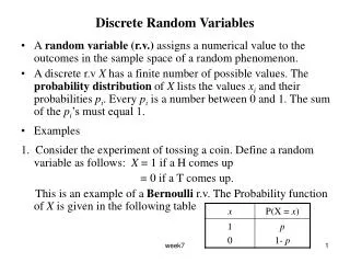
Discrete Random Variables: The Binomial Distribution. Bernoulli’s trials. J. Bernoulli (1654-1705) analyzed the idea of repeated independent trials for discrete random variables that had two possible outcomes: success or failure

E N D
Discrete Random Variables: The Binomial Distribution
Bernoulli’s trials • J. Bernoulli (1654-1705) analyzed the idea of repeated independent trials for discrete random variables that had two possible outcomes: success or failure • In his notation he wrote that the probability of success is denoted by p and the probability of failure is denoted by q or 1-p
Binomial distribution • The binomial distribution is just n independent individual (Bernoulli) trials added up. • It is the number of “successes” in n trials. • The sum of the probabilities of all the independent trials totals 1. • We can define a ‘success’ as a ‘1’, and a failure as a ‘0’.
Binomial distribution probability of success • “x” is a binomial distribution if its probability function is: • Examples (note – success/failure could be switched!): probability of failure
Binomial distribution • The binomial distribution is just n independent ‘Bernoulli trials’ added up • It requires that the trials be done “with replacement” ex. testing bulbs for defects: • Let’s say you make many light bulbs • Pick one at random, test for defect, put it back • Repeat several times • If there are many light bulbs, you do not have to replace (it won’t make a significant difference) • The result will be the binomial probability of a defective bulb (#defective total sample).
Binomial distribution - formula • Let’s figure out a binomial random variable’s probability function or formula • Suppose we are looking at a binomial with n=3 (ex. 3 coin flips; ‘heads’ is a ‘success’) • We will start with ‘all tails’ P(x=0): • Can happen only one way: 000 • Which is: (1-p)(1-p)(1-p) • Simplified: (1-p)3
Binomial distribution - formula • Let’s figure out a binomial probability function (for n = 3) • This time we want 1 success plus 2 failures (ex. 1 heads + 2 tails, or P(x=1)): • This can happen three ways: 100, 010, 001 • Which is: p(1-p)(1-p)+(1-p)p(1-p)+(1-p)(1-p)p • Simplified: 3p(1-p)2
Binomial distribution - formula • Let’s figure out a binomial probability function (for n = 3) • We want 2 ‘successes’ P(x=2): • Can happen three ways: 110, 011, 101, or… • pp(1-p)+(1-p)pp+p(1-p)p, which simplifies to.. • 3p2(1-p)
Binomial distribution - formula • Let’s figure out a binomial probability function (n = 3) • We want all 3 ‘successes’ P(x=3): • This can happen only one way: 111 • Which we represent as: ppp • Which simplifies to: p3
Binomial distribution - formula • Let’s figure out a binomial probability function – in summary, for n = 3, we have: P(x) (Where x is the number of successes; ex. # of heads) The sum of these expressions is the binomial distribution for n=3. The resulting equation is an example of the Binomial Theorem.
Binomial distribution - formula • A quick review of the Binomial Theorem: • If we use q for (1 – p), then… • p3 + 3p2q +3pq2 + q3 = (p + q)3 • which is an example of the formula: (a + b)n = ____________________ (if you forget it, check it in your text)
Binomial distribution - formula • Let’s figure out a binomial r.v.’s probability function (the quick way to compute the sum of the terms on the previous slide) - now here’s the formula… • In general, for a binomial: (the # of x successes with probability p in n trials)
Binomial distribution - formula • Which can be written as: orP(x) = nCxpx(1 – p)n-x • This formula is often called the general term of the binomial distribution.
Expected Value • The expected value of a binomial distribu-tion equals the probability of success (p) for n trials: • E(X) also equals the sum of the probabilities in the binomial distribution.
Binomial distribution - Graph • Typical shape of a binomial distribution: • Symmetric, with total P(x) = 1 Note: this is a theoretical graph – how would an experimental one be different? P x
Binomial distribution - example • A realtor claims that he ‘closes the deal’ on a house sale 40% of the time. • This month, he closed 1 out of 10 deals. • How likely is his claim of 40% if he only completed 1/10 of his deals this month?
Binomial distribution - example • By using the binomial distribution function, it’s possible to check if his assessment of his abilities (i.e. 40% ‘closes’) is likely: P(0 deals)=
Binomial distribution - example • So it seems pretty unlikely that his assess-ment of his abilities is right: • The probability of closing 1 or fewer deals out of 10 if (as he claims) he closes deals 40% of the time is less than 5% or less than 1/20. • What % of ‘closes’ do you think would have the highest probability in this distribution, if his claim was right?
Binomial distribution - example • Now see if you can determine the expected number of closings if he had 12 deals this month, assuming 40% success. • We need the values of n (= ___) and of p (= ____). • E(X) = np = ______ - this means that we would expect him to close about _____ deals, if his claim is correct. [End of first example.]
Binomial Distribution – ex. 2 • Alex Rios has a batting average of 0.310 for the season. In last night’s game, he had 4 at bats. What are the chances he had 2 hits? • You try this one! First ask 3 questions…
Binomial Distribution – ex. 2 • Is ‘getting a hit’ a discrete random variable? • Is this a Bernoulli trial? How would you define a “success” and a “failure”? • Is each time at bat an independent event? • If you can answer ‘yes’ to the three questions above, then you can use the binomial distribution formula to answer the problem.
Binomial Distribution – ex. 2 • First determine the following values: • The number of trials (Alex is at bat __ times) – this is the value of n • The probability of success (Alex’s average is ___) – this is p • The probability of ‘failure’: 1 – p = ___ • The # of successes asked for (his chances of getting ___ hits) – this is x • Now you can use the formula:
Binomial Distribution – ex. 2 • Put in the values from the previous screen, and discuss your answers. [pause here] • Did you get P(2) = 0.275? • Is 2 the most likely number of hits for Alex last night? How about 1 or 3? • P(0 or 1 or 2 or 3 or 4 hits) = _____?
Hypergeometric distribution • What happens if you have a situation in which the trials are not independent (this most often happens due to not replacing a selected item). • Each trial must result in success or failure, but the probability of success changes with each trial.
Hypergeometric distribution • Consider taking a sample from a population, and testing each member of the sample for defects. • Do this sampling without replacement. • As long as the sample is small compared to the population, this is close to binomial. • But if the sample is large compared to the population, this is a hypergeometric dist.
Hypergeometric dist. - formula • A hypergeometric distribution differs from binomial ones since it has dependent trials. • Probability of x successes in r dependent trials, with number of successes a out of a total of n possible outcomes:
Hypergeometric dist. - formula • The full version of this formula is: • Expected Value – the average probability of a success is the ratio of success overall (a/n) times r trials: