Download
1 / 41
410 likes | 413 Views
Binomial Random Variables. Binomial Probability Distributions. Binomial Random Variables. Through 2/24/2011 NC State’s free-throw percentage is 69.6% (146 th out 345 in Div. 1). If in the 2/26/2011 game with GaTech, NCSU shoots 11 free-throws, what is the probability that:

E N D
Binomial Random Variables Binomial Probability Distributions
Binomial Random Variables • Through 2/24/2011 NC State’s free-throw percentage is 69.6% (146th out 345 in Div. 1). • If in the 2/26/2011 game with GaTech, NCSU shoots 11 free-throws, what is the probability that: • NCSU makes exactly 8 free-throws? • NCSU makes at most 8 free throws? • NCSU makes at least 8 free-throws?
“2-outcome” situations are very common • Heads/tails • Democrat/Republican • Male/Female • Win/Loss • Success/Failure • Defective/Nondefective
Probability Model for this Common Situation • Common characteristics • repeated “trials” • 2 outcomes on each trial • Leads to Binomial Experiment
Binomial Experiments • n identical trials • n specified in advance • 2 outcomes on each trial • usually referred to as “success” and “failure” • p “success” probability; q=1-p “failure” probability; remain constant from trial to trial • trials are independent
Binomial Random Variable • The binomial random variable X is the number of “successes” in the n trials • Notation: X has a B(n, p) distribution, where n is the number of trials and p is the success probability on each trial.
Examples • Yes; n=10; success=“major repairs within 3 months”; p=.05 • No; n not specified in advance • No; p changes • Yes; n=1500; success=“chip is defective”; p=.10
Rationale for the Binomial Probability Formula n! P(x) = •px•qn-x (n –x )!x! Number of outcomes with exactly x successes among n trials
Binomial Probability Formula n! P(x) = •px•qn-x (n –x )!x! Probability of x successes among n trials for any one particular order Number of outcomes with exactly x successes among n trials
The sum of all the areas is 1 p(5)=.246 is the area of the rectangle above 5 Graph of p(x); x binomial n=10 p=.5; p(0)+p(1)+ … +p(10)=1 Think of p(x) as the area of rectangle above x
Example A production line produces motor housings, 5% of which have cosmetic defects. A quality control manager randomly selects 4 housings from the production line. Let x=the number of housings that have a cosmetic defect. Tabulate the probability distribution for x.
Solution • (i) D=defective, G=good outcomexP(outcome) GGGG 0 (.95)(.95)(.95)(.95) DGGG 1 (.05)(.95)(.95)(.95) GDGG 1 (.95)(.05)(.95)(.95) : : : DDDD 4 (.05)4
Solution x 0 1 2 3 4 p(x) .815 .171475 .01354 .00048 .00000625
Example (cont.) x 0 1 2 3 4 p(x) .815 .171475 .01354 .00048 .00000625 • What is the probability that at least 2 of the housings will have a cosmetic defect? P(x 2)=p(2)+p(3)+p(4)=.01402625
Example (cont.) x 0 1 2 3 4 p(x) .815 .171475 .01354 .00048 .00000625 • What is the probability that at most 1 housing will not have a cosmetic defect? (at most 1 failure=at least 3 successes) P(x 3)=p(3) + p(4) = .00048+.00000625 = .00048625
9, 10, 11, … , 20 Using binomial tables; n=20, p=.3 • P(x 5) = .4164 • P(x > 8) = 1- P(x 8)= 1- .8867=.1133 • P(x < 9) = ? • P(x 10) = ? • P(3 x 7)=P(x 7) - P(x 2) .7723 - .0355 = .7368 8, 7, 6, … , 0 =P(x 8) 1- P(x 9) = 1- .9520
Binomial n = 20, p = .3 (cont.) • P(2 < x 9) = P(x 9) - P(x 2) = .9520 - .0355 = .9165 • P(x = 8) = P(x 8) - P(x 7) = .8867 - .7723 = .1144
Color blindness The frequency of color blindness (dyschromatopsia) in the Caucasian American male population is estimated to be about 8%. We take a random sample of size 25 from this population. We can model this situation with a B(n = 25, p = 0.08) distribution. • What is the probability that five individuals or fewer in the sample are color blind? Use Excel’s “=BINOMDIST(number_s,trials,probability_s,cumulative)” P(x≤ 5) = BINOMDIST(5, 25, .08, 1) = 0.9877 • What is the probability that more than five will be color blind? P(x> 5) = 1 P(x≤ 5) =1 0.9877 = 0.0123 • What is the probability that exactly five will be color blind? P(x= 5) = BINOMDIST(5, 25, .08, 0) = 0.0329
B(n = 25, p = 0.08) Probability distribution and histogram for the number of color blind individuals among 25 Caucasian males.
What are the mean and standard deviation of the count of color blind individuals in the SRS of 25 Caucasian American males? µ = np = 25*0.08 = 2 σ = √np(1 p) = √(25*0.08*0.92) = 1.36 What if we take an SRS of size 10? Of size 75? µ = 10*0.08 = 0.8 µ = 75*0.08 = 6 σ = √(10*0.08*0.92) = 0.86 σ = √(75*0.08*0.92) = 2.35 p = .08 n = 10 p = .08 n = 75
Recall Free-throw question • Through 2/24/11 NC State’s free-throw percentage was 69.6% (146th in Div. 1). • If in the 2/26/11 game with GaTech, NCSU shoots 11 free-throws, what is the probability that: • NCSU makes exactly 8 free-throws? • NCSU makes at most 8 free throws? • NCSU makes at least 8 free-throws? • n=11; X=# of made free-throws; p=.696 p(8)= 11C8 (.696)8(.304)3 • P(x ≤ 8)=.697 • P(x ≥ 8)=1-P(x≤7) =1-.4422 = .5578
Recall from beginning of Lecture Unit 4: Hardee’s vs The Colonel • Out of 100 taste-testers, 63 preferred Hardee’s fried chicken, 37 preferred KFC • Evidence that Hardee’s is better? A landslide? • What if there is no difference in the chicken? (p=1/2, flip a fair coin) • Is 63 heads out of 100 tosses that unusual?
Use binomial rv to analyze • n=100 taste testers • x=# who prefer Hardees chicken • p=probability a taste tester chooses Hardees • If p=.5, P(x 63) = .0061 (since the probability is so small, p is probably NOT .5; p is probably greater than .5, that is, Hardee’s chicken is probably better).
Recall: Mothers Identify Newborns • After spending 1 hour with their newborns, blindfolded and nose-covered mothers were asked to choose their child from 3 sleeping babies by feeling the backs of the babies’ hands • 22 of 32 women (69%) selected their own newborn • “far better than 33% one would expect…” • Is it possible the mothers are guessing? • Can we quantify “far better”?
Use binomial rv to analyze • n=32 mothers • x=# who correctly identify their own baby • p= probability a mother chooses her own baby • If p=.33, P(x 22)=.000044 (since the probability is so small, p is probably NOT .33; p is probably greater than .33, that is, mothers are probably not guessing.
Geometric Random Variables • Geometric Probability Distributions • Through 2/24/2011 NC State’s free-throw percentage was 69.6 (146th of 345 in Div. 1). In the 2/26/2011 game with GaTech what was the probability that the first missed free-throw by the ‘Pack occurs on the 5th attempt?
Binomial Experiments • n identical trials • n specified in advance • 2 outcomes on each trial • usually referred to as “success” and “failure” • p “success” probability; q=1-p “failure” probability; remain constant from trial to trial • trials are independent • The binomial rv counts the number of successes in the n trials
The Geometric Model • A geometric random variable counts the number of trials until the first success is observed. • A geometric random variable is completely specified by one parameter, p, the probability of success, and is denoted Geom(p). • Unlike a binomial random variable, the number of trials is not fixed
The Geometric Model (cont.) Geometric probability model for Bernoulli trials: Geom(p) p = probability of success q = 1 – p = probability of failure X = # of trials until the first success occurs p(x) = P(X = x) = qx-1p, x = 1, 2, 3, 4,…
The Geometric Model (cont.) • The 10% condition: the trials must be independent. If that assumption is violated, it is still okay to proceed as long as the sample is smaller than 10% of the population. Example: 3% of 33,000 NCSU students are from New Jersey. If NCSU students are selected 1 at a time, what is the probability that the first student from New Jersey is the 15th student selected?
Example The American Red Cross says that about 11% of the U.S. population has Type B blood. A blood drive is being held in your area. • How many blood donors should the American Red Cross expect to collect from until it gets the first donor with Type B blood? Success=donor has Type B blood X=number of donors until get first donor with Type B blood
Example (cont.) The American Red Cross says that about 11% of the U.S. population has Type B blood. A blood drive is being held in your area. • What is the probability that the fourth blood donor is the first donor with Type B blood?
Example (cont.) The American Red Cross says that about 11% of the U.S. population has Type B blood. A blood drive is being held in your area. • What is the probability that the first Type B blood donor is among the first four people in line?
Example Shanille O’Keal is a WNBA player who makes 25% of her 3-point attempts. • The expected number of attempts until she makes her first 3-point shot is what value? • What is the probability that the first 3-point shot she makes occurs on her 3rd attempt?
Question from first slide • Through 2/24/2011 NC State’s free-throw percentage was 69.6%. In the game with GaTech what was the probability that the first missed free-throw by the ‘Pack occurs on the 5th attempt? “Success” = missed free throw Success p = 1 - .696 = .304 p(5) = .6964 .304 = .0713