Download
1 / 27
270 likes | 287 Views
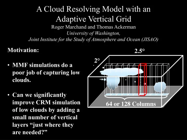
A Cloud Resolving Model with an Adaptive Vertical Grid Roger Marchand and Thomas Ackerman University of Washington, Joint Institute for the Study of Atmosphere and Ocean (JISAO). Depiction of Multi-scale Modeling Framework (MMF). 2.5 °. Motivation:

E N D
A Cloud Resolving Model with an Adaptive Vertical GridRoger Marchand and Thomas Ackerman University of Washington, Joint Institute for the Study of Atmosphere and Ocean (JISAO) Depiction of Multi-scale Modeling Framework (MMF) 2.5° • Motivation: • MMF simulations do a poor job of capturing low clouds. • Can we significantly improve CRM simulation of low clouds by adding a small number of vertical layers “just where they are needed?” 2° 64 or 128 Columns
Control • 4 km horizontal • 64 columns • 26 vertical layers • Test A • 1 km horizontal • 64 & 128 columns • 26 vertical layers • Test B • 1 km horizontal • 64 columns • 52 vertical layers Sensitivity of low cloud amount to CRM resolution
What kind of vertical resolution do we need ?DYCOMS II + Set up as per Stevens et. al (2005) + Simulations with SAM 6.5 (Kharoutdinov)
Adaptive Vertical Grid Simulation of DYCOMS-II • Modified SAM: • Vertical layers are addressed by an index array (data can be stored vertically in any order) • One can add or remove a layer (Mass and Energy are conserved). • Criteria: Examine ratio of SGS/Total vertical water flux, (Threshold to add << to remove)
Atlantic Strotocumuls Transition Experiment (ASTEX) following Duynkerke et al. (1999)
Adaptive Vertical Grid Simulation of ASTEX – Potential Temperature Criteria
Adaptive Vertical Grid Simulation of ASTEX – SGS/Total vertical water flux criteria
Adaptive Vertical Grid Simulation of ASTEX – Buoyancy Flux & TKE Fixed Vertical Grid Adaptive Vertical Grid
Adaptive Vertical Grid Simulation of ASTEX – Ratio SGS/Total vertical water flux & TKE criteria
Atlantic Trade Wind Experiment (ATEX) following Stevens et al. (2001)
Atlantic Trade Wind Experiment (ATEX) - SGS/Total vertical water flux criteria
Closing Remarks • Starting with modest vertical resolution (100 m), SAM-AVG is able to simulate DYCOMS-II, ASTEX, and ATEX reasonably well compared with model runs using fine vertical resolution everywhere. • Adding vertical levels only at cloud-top may not always be sufficient • DYCOMS-II need layers and cloud top to model entrainment well • ATEX need layers primarily at cloud top to get cloud/LW feedback • ASTEX need layers below cloud to capture buoyancy from surface/sub-cloud layers • More work is needed to optimize criteria for adding and removing vertical layers --- suggestions please ! • Would like to identify case studies with • Low/less sensitivity to the model initialization /spin-up … • “Confront” results with observations … • suggestions are welcome.
Atlantic Trade Wind Experiment (ATEX) - Potential Temperature Criteria
MISR Observational attributes Polar Orbit with 400-km swath Contiguous zonal coverage: 9 days at equator 2 days at poles 275 m sampling 7 minutes to observe each scene at all 9 angles 9 CCD pushbroom cameras 9 view angles at Earth surface: 70.5º. 60.0º, 45.6º, 26.1º forward of nadir nadir 26.1º, 45.6º, 60.0º, 70.5º backward of nadir 4 spectral bands at each angle:c 446,558,672,866 nm 14-bit digitization On-board calibration system
Satellite First view angle Apparent position height above the surface Surface Second view angle (no cloud motion) position in first image Surface Parallax : Apparent change in position Second view angle (with cloud motion) Apparent position in first image Surface Cloud Motion + Parallax Stereo-imaging • A significant advantage of the MISR CTH retrieval is that the technique is purely geometric and has little sensitivity to the sensor calibration. • The retrieval has been the focus of several studies including Marchand et al. (2007), Naud et al. (2002, 2004, and 2005a,b), Seiz et al. (2005), Marchand et al. (2001).
Summary of Low Cloud Response • Increasing horizontal resolution from 4 km to 1 km resulted in a reduction of low cloud amount. • Much (but not all) due to dissipation of “stratofogulus” • Generally, little change in amount of low cloud with optical depths less than 10. • Increasing horizontal resolution and vertical resolution to 52 levels (50 in CRM) resulted in … • Small increase in the amount of low-level cloud relative to the simulations with 4 km horizontal resolution. • There is an increase in the amount of cloud with optical depths less than 10, bringing the model results into better agreement with MISR observational data. • Stratocumulus zones show a significant improvement in cloud top height. … • Nonetheless, the total amount of model low cloud remains too low and there is still too much low cloud with optical depths larger than 23 (the largest two optical-depth bins). • Analysis make use of a “MISR simulator”. This code has been added to the suite of instrument simulators in the CFMIP Observation Simulator Package (COSP). http://cfmip.metoffice.com/COSP.html