Download

1 / 41
410 likes | 573 Views
Model Selection Problems in Image Analysis. Mário A. T. Figueiredo Department of Electrical and Computer Engineering Instituto Superior Técnico Technical University of Lisbon PORTUGAL. www.lx.it.pt/~mtf. What is model selection?. ...to which we want to fit a polynomial.

E N D
Model Selection Problems in Image Analysis Mário A. T. Figueiredo Department of Electrical and Computer Engineering Instituto Superior Técnico Technical University of Lisbon PORTUGAL www.lx.it.pt/~mtf
What is model selection? ...to which we want to fit a polynomial. Question: which order? “underfitting” “overfitting” How to identify the underlying trend of the data, ignoring the noise? Some experimental data...
Outline 1. What is model selection ? 2. Introduction and some motivating examples 3. Bayesian model selection 4. Minimum description length (MDL) 5. Implicit model selection via sparseness priors 6. Concluding remarks Examples are shown along the way...
Motivating example Goal: fit some function (e.g., a polynomial) Unknown parameters: Any estimation criterion, for fixed k Objective function (e.g., mean squared error, likelihood,...) Parameter space of orderk, e.g., y Observed data x In general, k may not be the number of parameters, just some “model order”
Motivating example No, if the parameter spaces are nested: Can we use the minimized criterion for model selection? Example: for every quadratic polynomial, there is an equivalentthird order polynomial; simply set to zero the extra coefficient. We may also have increasingly “complex” models, not necessarily nested.
Examples in signal/image/pattern analysis inference spline representationof a contour, with k control points Contour estimation y observed image Model selection question: how many control points ? (how simple/smooth?)
Examples in signal/image/pattern analysis inference image segmentation into k regions Image segmentation y observed image Model selection question: how many regions ?
Probabilistic formulation Observation model (likelihood function): For maximum likelihood (ML) estimation, ...the maximized likelihood is useless for model selection. ML estimation (for fixed k) is very well studied model selection Choosing k Unknownquantities/parameters: Observed data:
Ockham’s razor Implicit, via sparsity penalties Bayesian Information theoretic(MDL, MML) Preference for simpler models is a spin-off. Built-in Ockham’s razor Parsimony is built intothe inference criteria (“short code-length”) Preference for models with many zero parametersis imposed When talking about model selection, “Ockham’s razor” comes to mind. “Ockham’s razor” principle (XIVth century) “a plurality should not be posited except where necessary” ...that is, we should prefer “simpler” models. Model selection approaches Other methods: cross-validation, statistical tests, ...not considered here.
Bayesian approach and k Likelihood function: A priori knowledge (prior) Bayes law Posterior: If goal is only to select k (don’t care about q ), the relevant posterior is Unknowns:
Bayesian model selection marginal likelihood ..the key to the built-in parsimony of the Baysian approach [MacKay, 1991]. If the model is too complex, is large in a small regionbut very small almost everywhere else. If the model is too simple, is never very large. Maximum a posteriori (MAP) model selection: The marginal likelihood promotes a balance between data-fit and complexity.
Bayesian model selection: Laplace-type approximations Laplace-type approximation: maximum likelihood estimate Bayesian inference criterion (BIC), [Schwartz, 1978]. with k with k penalizes larger k Conditions: smooth prior, regularity of the likelihood, large n Order-penalized maximum likelihood.
BIC: Example estimate truth 3 Back to the polynomial toy example
Penalized likelihood criteria If Only depends on the model dimension Structural risk minimization type criteria,i.e., choose the best model from each class (k),then select among these models.Examples: BIC, SRM, classical MDL, etc... General form of penalized likelihood criteria: Complexity penalty Many instances: BIC, NIC, AIC, SIC, MDL, MML, NML, ...
The minimum description length (MDL) criterion good model encoder Rationale: short code long codebad model compressed data code lengthmodel adequacy Several flavors: [Rissanen 1978, 1987] [Rissanen 1996] [Wallace and Freeman, 1987] decoder Introduction: observed data
Two-part code MDL However, both k and are unknown to the decoder observed data encoder estimator coded data decoder MDL criterion: extract Given , the shortest codelength for is [Shannon, 1948]. A maximum penalized likelihood criterion
MDL criterion: coding the parameters Real-valued parameters: how to code with a finite number of bits ? truncated to finite precision Under regularity conditions, can be shown that optimal precision, when MDL = BIC This is the “standard” MDL; there are more recent/refined versions (more later).
Image analysis example: contour estimation observed image contour description y a statistical model for the inside, observation mechanism ...another one for the outside other parameters Examples: Gaussians of different means and/or variances; Rayleigh of different variances (ultrasound images); different textures. [Figueiredo, Leitão, 1992], [Figueiredo, Leitão, Jain, 1997, 2000].
Spline contour representation contourcontrol points contour control points matrix with periodic B-spline basis functions Fewer control points simpler (smoother) shape Model selection:k = ? Approach: MDL/BIC
Some results k = 9 k = 13 k = 7 same variance, different means k = 11 description length k = 5 [Figueiredo, Leitão, Jain, 1997, 2000].
The importance of the region-based model initialization same mean, different variances/textures This contour could never be estimated withan edge-based (snake-type) approach.
Poisson field segmentation A Poissonian image Model:k regions/segments of constant mean: A sequence of Poisson counts (e.g., X-ray astronomical data) Model selection question:k = ?
MDL for Poisson segmentation Example -250 -255 -260 -265 -270 -275 1 50 100 150 200 i model i segment at location i Fully Bayes / MDL-optimal criterion. No user-defined thresholds, no approximations. no segmentation model 0 Poisson model: parameter estimates are rational numbers No quantization needed Elementary problem: segmenting a sequence into two parts.
Non-incomplete MDL for Poisson segmentation true intensity function Example: estimate Observed counts 40 30 20 10 0 200 400 600 [Figueiredo and Nowak, 1999, 2000] What about multiple change points ? Simply take each segment and re-apply the criterion (recursively)
Non-incomplete MDL for Poisson image segmentation 1 - competing models: no segmentation, all possible 4-segmentations, and all possible 2-segmentations ky Ny 1 Nx kx In 2D, we look for the best (if any) segmentation into two/four rectangles: Same multinomial-based criterion: To fully segment an image: apply criterion recursively.
Segmenting Poisson images: synthetic example counts intensity estimates 250x250 pixels/bins segmentation True intensities [Figueiredo and Nowak, 1999, 2000]
Segmenting Poisson images: real example adaptive recursive partioning (ARP) multi-look SAR Approximated by Poisson model, by moment matching. Can also develop non-incomplete MDL criterion for Gaussian data, but need asymptotic approximation [Ndili, Figueiredo, Nowak, 2001].
Implicit model selection via sparseness many zeros “Model selection” in the sense that will favor sparse estimates. Typical choice: Take “full model” and encourage redundant parameters to go to zero. We drop explicit mention of k This can be seen as a MAP estimate, with prior Laplacian prior LASSO regression [Tibshirani, 1996], basis pursuit [Chen, Donoho, Saunders, 1995], image denoising and restoration [Figueiredo, Nowak, 2001, 2003]. sparse linear regression and probit regression [Figueiredo, 2001, 2003], logistic regression [Krishnapuram, Figueiredo, Carin, Hartemink, 2004].
Sparseness inducing nature of Laplacian-type priors Compare behavior at the origin: Laplacian: “reward” derivative keeps increasing as estimate approaches zero. Gaussian Laplacian Gaussian: “reward” increase slows down as estimate approaches zero.
Linear observation models Many problems have this form; I’ll focus on: - Image denoising; - Image restoration (deblurring). - Image super-resolution.
Linear observation models and sparseness prior problem Least squares cost function A more natural “model selection” criterion: problem Number of non-zero elements in Very recent results show that and are closely related (under conditions) [Tropp 2003], [Donoho, Elad, Temlyakov, 2003], [Donoho, 2004]
Example: wavelet-based image denoising Observation model Original image H = W, matrix with (maybe redundant) wavelet basis Natural images can be represented by very sparse (many zeros). , a noisy image Closed form (fast) solution with or Jeffreys prior
Example: wavelet-based image denoising Denoised image State-of-the-art results in 2001, using Jeffreys prior [Figueiredo and Nowak, 2001]. Noisy image
Example: wavelet-based image debluring Observation model Original image Blur matrix In this case, Sparseness prior , a noisy blurred image Can’t be solved in closed form, due to BW. EM algorithm, seeing x as missing data[Figueiredo and Nowak, 2002, 2003].
Example: image debluring restored blurred Uniform 9x9 blur (BSNR = 40dB)
Example: image debluring Separable, blur with [1,4,6,4,1] restored blurred
Deblurring aerial images Restored image[Jalobeanu, Nowak, Zerubia, Figueiredo, 2002]
Concluding remarks Model selection permeates image analysis and processing Natural formulation in a Bayesian framework Complexity penalties also in MDL framework Order can also be penalized implicitly via sparseness priors Examples: contour estimation, signal/image segmentation, wavelet-based image denoising, wavelet-based image deblurring..