Download
1 / 33
330 likes | 421 Views
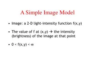
Image Model. Dr. Samir H. Abdul-Jauwad Electrical Engineering Department King Fahd University of Petroleum & Minerals. A Simple Image Model. Image: a 2-D light-intensity function f(x,y) The value of f at (x,y) the intensity (brightness) of the image at that point 0 < f(x,y) < .

E N D
Image Model Dr. Samir H. Abdul-Jauwad Electrical Engineering Department King Fahd University of Petroleum & Minerals
A Simple Image Model • Image: a 2-D light-intensity function f(x,y) • The value of f at (x,y) the intensity (brightness) of the image at that point • 0 < f(x,y) <
A Simple Image Model • Nature of f(x,y): • The amount of source light incident on the scene being viewed • The amount of light reflected by the objects in the scene
A Simple Image Model • Illumination & reflectance components: • Illumination: i(x,y) • Reflectance: r(x,y) • f(x,y) = i(x,y) r(x,y) • 0 < i(x,y) < and 0 < r(x,y) < 1 (from total absorption to total reflectance)
A Simple Image Model • Sample values of r(x,y): • 0.01: black velvet • 0.93: snow • Sample values of i(x,y): • 9000 foot-candles: sunny day • 1000 foot-candles: cloudy day • 0.01 foot-candles: full moon
A Simple Image Model • Intensity of a monochrome image f at (xo,yo): gray level l of the image at that point l=f(xo, yo) • Lmin≤ l ≤ Lmax • Where Lmin: positive Lmax: finite
A Simple Image Model • In practice: • Lmin = imin rmin and • Lmax = imax rmax • E.g. for indoor image processing: • Lmin≈ 10 Lmax ≈ 1000 • [Lmin, Lmax] : gray scale • Often shifted to [0,L-1] l=0: black l=L-1: white
Sampling & Quantization • The spatial and amplitude digitization of f(x,y) is called: • image sampling when it refers to spatial coordinates (x,y) and • gray-level quantization when it refers to the amplitude.
Sampling & Quantization Image Elements (Pixels) Digital Image
Sampling & Quantization • Important terms for future discussion: • Z: set of real integers • R: set of real numbers
Sampling & Quantization • Sampling: partitioning xy plane into a grid • the coordinate of the center of each grid is a pair of elements from the Cartesian product Z x Z (Z2) • Z2 is the set of all ordered pairs of elements (a,b) with a and b being integers from Z.
Sampling & Quantization • f(x,y) is a digital image if: • (x,y) are integers from Z2 and • f is a function that assigns a gray-level value (from R) to each distinct pair of coordinates (x,y) [quantization] • Gray levels are usually integers • then Z replaces R
Sampling & Quantization • The digitization process requires decisions about: • values for N,M (where N x M: the image array) and • the number of discrete gray levels allowed for each pixel.
Sampling & Quantization • Usually, in DIP these quantities are integer powers of two: N=2n M=2m and G=2k number of gray levels • Another assumption is that the discrete levels are equally spaced between 0 and L-1 in the gray scale.
Sampling & Quantization • If b is the number of bits required to store a digitized image then: • b = N x M x k (if M=N, then b=N2k)
Sampling & Quantization • How many samples and gray levels are required for a good approximation? • Resolution (the degree of discernible detail) of an image depends on sample number and gray level number. • i.e. the more these parameters are increased, the closer the digitized array approximates the original image.
Sampling & Quantization • How many samples and gray levels are required for a good approximation? (cont.) • But: storage & processing requirements increase rapidly as a function of N, M, and k
Sampling & Quantization • Different versions (images) of the same object can be generated through: • Varying N, M numbers • Varying k (number of bits) • Varying both
Sampling & Quantization • Isopreference curves (in the Nm plane) • Each point: image having values of N and k equal to the coordinates of this point • Points lying on an isopreference curve correspond to images of equal subjective quality.
Sampling & Quantization • Conclusions: • Quality of images increases as N & k increase • Sometimes, for fixed N, the quality improved by decreasing k (increased contrast) • For images with large amounts of detail, few gray levels are needed
Nonuniform Sampling & Quantization • An adaptive sampling scheme can improve the appearance of an image, where the sampling would consider the characteristics of the image. • i.e. fine sampling in the neighborhood of sharp gray-level transitions (e.g. boundaries) • Coarse sampling in relatively smooth regions • Considerations: boundary detection, detail content
Nonuniform Sampling & Quantization • Similarly: nonuniform quantization process • In this case: • few gray levels in the neighborhood of boundaries • more in regions of smooth gray-level variations (reducing thus false contours)