Download
1 / 38
380 likes | 501 Views
Surface Skin Temperature, Soil Moisture, and Turbulent Fluxes in Land Models. Xubin Zeng, Mike Barlage, Mark Decker, Jesse Miller, Cindy Wang, Jennifer Wang Dept of Atmospheric Sciences University of Arizona Tucson, AZ 85721, USA.

E N D
Surface Skin Temperature, Soil Moisture, and Turbulent Fluxes in Land Models Xubin Zeng, Mike Barlage, Mark Decker, Jesse Miller, Cindy Wang, Jennifer Wang Dept of Atmospheric Sciences University of Arizona Tucson, AZ 85721, USA (a) A revised form of Richards equation (b) CLM3 simulation versus MODIS skin TConsistent (c) Treatment of turbulence below and above canopy as well as snow burial of canopy (d) Vegetation and snow albedo data
Decker and Zeng (2007)
CLM3 offline tests over Sahara, southwest US and Tibet For July 1-5, 2003.
Cs = Cs,soil W + Cs,veg (1 – W) Zeng et al. (2005) W = exp(– LAI)
Dickinson et al. (2006)
Thought experiment: What would be the land zo and d If above-ground biomass disappears? CLM3 deficiency: zo and d depend on vegetation type only Solution: de = d V + (1 – V) dg ln (zoc,e) = V ln(zoc) + (1 – V) ln (zog) V = (1 – exp[-β min(Lt, Lcr)])/(1 – exp[- β Lcr])
Figure C. 1 CLM3-simulated snow depth and surface fluxes from Jan. 11-13, 1996 over a boreal grassland site in Canada. Both simulation with new formulation of fv,sno and simulation with standard CLM3 are shown (52.16ºN, 106.13ºW ).
Wang and Zeng (2007) Figure C.2 The same simulation as in Fig. C. 1 but for averaged diurnal cycles of winter time (Dec. 1995, Jan. and Feb. 1996).
Figure C.4 (a) Ten-year averaged DJF differences of Tg between CLM3 with Eq.(C. 3) and the standard CLM3 global offline simulations, and (b) ten-year averaged annual cycle of Tgdifference over Alaska (59-72ºN, 170-140ºW).
NCAR/CLM3: FVC(x,y), LAI(x,y,t) NCEP/Noah: GVF(x,y,t),LAI=Const Validation: 1-3m spy sat data, 1-5m aircraft data, 30m Landsat data, Surface survey data Zeng et al. (2000)
Data Impact Barlage and Zeng (2004)
NLDAS GVF Data Noah 1/8 degree monthly MODIS 2km 16-day Miller et al. (2006)
NLDAS GVF Results grass • Addition of new GVF dataset results in an increase of transpiration (up to 35W/m2) and canopy evaporation (up to 8W/m2) • Balanced by a decrease in ground evaporation (up to 20W/m2) • Overall increase in LHF(up to 20W/m2) is balanced by decreases in SHF(up to 10W/m2) and Lwup(5W/m2) crop Miller et al. (2006)
Albedo NDSI NDVI Land cover Individual bands Red: NN filled Blue: LAT filled Green: > 0.84 MODIS versus Noah maximum snow albedo data Barlage et al. (2005)
Impact on NLDAS Offline Noah Tests Barlage et al. (2005)
Application of MODIS Maximum Snow Albedo to WRF-NMM/NOAH • up to 0.5 C decreases in 2-m Tair in regions of significant albedo change • > 0.5 C increase in 2-m Tair in several regions Barlage et al. (2007)
Summary • Skin temperature and turbulent fluxes are all strongly affected by the treatment of below and above-canpy turbulence and snow burial • They are also affected by green vegetation cover data as well as maximum snow albedo data • While Terra/Aqua MODIS provides 4 skin Ts measurements a day, its use without constraint from Tair requires additional efforts • The revised Richards equation should be used for land models for improved simulations of soil moisture and fluxes
Suggestions on LANDFLUX • Try to reach some consensuses on the land boundary data to be used • Identify flux tower sites with relatively comprehensive data over different climate regimes to set up minimum criteria for land models or model components to meet • Try to use land-atmosphere constrained land and atmospheric forcing data
Model Run • Model Alterations • New Richards equation • Including new bottom boundary condition • NO TUNABLE PARAMETERS • Soil texture constant with depth • Infiltration • Area of Saturated Fraction • 1984-2004 with Qian/Dai forcing
Comparison of CAM/CLM3 with the Terra and Aqua MODIS data
Fractional Vegetation Cover NCAR/CLM3: FVC(x,y), LAI(x,y,t) NCEP/Noah: GVF(x,y,t),LAI=Const Validation: 1-3m spy sat data, 1-5m aircraft data, 30m Landsat data, Surface survey data Histogram of evergreen Broadleaf tree NDVIveg = 0.69
Interannual variability and decadal trend of global fractional vegetation cover from 1982 to 2000 Zeng et al. (2003)
Maximum Snow Albedo in the NCEP Noah Land Model • Shading effect • Shadowing effect • LAI is difficult to measure in winter! • A = Asn fsn + Av(1-fsn) • Then the question is • (1) what is satellite • snow fraction? • (2) What is Asn?
Issue: Consistency of Cx below/within canopy Motivation: warm bias of 10 K in Tg in CCSM2 Below/within canopy in CLM Hg ~ Cs u* (Tg – Tva) Hf ~ Cf LAI u*0.5 (Tv – Tva) Cs = const in BATS, LSM, CLM2 Based on K-theory Cs ≈ 0.13 b exp(-0.9b)/[1 – exp(-2b/3)] b = f(LAI, stability)
Surface Skin Temperature, Soil Moisture, and Turbulent Fluxes in Land Models Xubin Zeng Mike Barlage, Mark Decker, Jesse Miller, Cindy Wang, Jennifer Wang Dept of Atmospheric Sciences University of Arizona Tucson, AZ 85721, USA
Turbulence • Energy Balance: Rnet + G + Ft + Fq ≈ 0 • Water Balance: P ≈ Fq + R • Turbulent fluxes Fx ~ Cx U (Xa – Xs) • Cx = f(Zom, Zot, stability) • X: temperaure, humidity, wind, trace gas • Consistent treatment of turbulence below and above • canopy as well as snow burial of canopy • Vegetation and snow albedo data • CAM3/CLM3 simulation versus MODIS skin T • A revised form of Richards equation