Download
1 / 34
560 likes | 1.35k Views
Chapter 9: Climate Sensitivity and Feedback Mechanisms . This chapter discusses: Climate feedback processes Climate sensitivity and climate feedback parameter Examples

E N D
Chapter 9: Climate Sensitivity and Feedback Mechanisms • This chapter discusses: • Climate feedback processes • Climate sensitivity and climate feedback parameter • Examples • (Materials are drawn heavily from D. Hartmann’s textbook and online materials by J.-Y. Yu of UCI. Guo-Yue Niu contributed significantly to the preparation of this lecture.)
Climate Feedback and Sensitivity Feedback is a circular causal process whereby some proportion of a system's output is returned (fed back) to the input. ΔQ input ΔQfinal Climate System output ΔT ΔTfinal ΔQfinal = ΔQ + ΔQfeedback ΔQfeedback can be either negative or positive ΔTfinal = ΔT + ΔTsensitivity
An objective measure of climate feedback and sensitivity The strength of a feedback depends on how sensitive the change in input (Q) responds to the change in output (T) : Feedback strength: λ = ΔQ / ΔT Climate sensitivity: λ-1 = ΔT / ΔQ 1. Positive values negative feedbacks, stable Negative values positive feedbacks, unstable λBB = 4σT3 = 3.75Wm-2K-1 2. The larger λ, the stronger feedback.
Stefan-Boltzmann feedback Outgoing longwave radiation: F = σT4 σ = 5.67x10⁻⁸ The strength of the feedback: λBB = ∂F / ∂T = 4σ T3 = 3.75 Wm-2K-1 1. A negative feedback, stable 2. 1K increase in T would increase F by 3.75 Wm-2 (see Fig. 9.1)
Water vapor feedback Clausius-Clapeyron relationship: es = f(T) 1% increase in T would increase 20% in es Water vapor is the principal greenhouse gases. The feedback strength: λv= – 1.7 Wm-2K-1 1. A positive feedback, unstable 2. Weaker than λBB 3. λBB + λv = 2.05 Wm-2K-1 (see Fig. 9.1)
Ice (snow) albedo feedback Striking contrast between ice-covered and ice-free surfaces In ice-covered regions, more solar energy reflected back to space: Feedback strength: λice= –0.6 Wm-2K-1 1. Positive feedback, unstable 2. λBB + λv + λice=1.45 Wm-2K-1
An example of climate feedback Global Temperature Anomalies ΔT Northern Hemisphere Snow Cover Anomalies ΔQ
Snow cover change Temperature change Chapin et al. (2005), Science 1. Decrease in snow-cover and snow season 2. Tundra trees Snow (ice)-albedo climate feedback
Total feedback λtotal =1.45 Wm-2K-1 Positive feedback negative feedback λtotal 3.75 Wm-2K-1 Doubling of atmospheric CO2 2.9 K Without ice-albedo feedback 2.0 K
−31 −48 −17 +15%
Cloud feedback • It is unclear what is the strength and even directions (negative or positive). From GCM simulations, λcloud = 0 ─ −0.8. • 2. Could effects can be either “umbrella” or “blanket”. • umbrella blanket Low cumulus clouds Negative feedback High cirrus clouds Positive feedback
Cloud feedback (con.) 3. It is uncertain whether an increased temperature will lead to increased or decreased cloud cover. 4. It is generally agreed that increased temperatures will cause higher rates of evaporation and hence make more water vapor available for cloud formation, the form (e.g., type, height, and size of droplets) which these additional clouds will take is much less certain.
Energy-balance climate models • Zero-dimensional EBMs • (1-α) S0 /4 = σTe4 shortwave in = Longwave out The surface T: Ts = Te + ΔT (greenhouse effects) The Erath: S0 = 1376 Wm-2, α = 0.3, Te= 255 K, Ts =288 K Venus: S0 = 2619 Wm-2, α = 0.7, Te = 242 K, greenhouse gases Ts = 730 K
Energy balance climate models (con.) 2. One-dimensional EBMs (Sellers and Budyko in 1969) Shortwave in = Transport out + Longwave out S(x) [1 - α(x) ] = C [ T(x) - Tm ] + [ A + B T(x) ] S(x) = the mean annual radiation incident at latitude (x) = S0/4*s(x) α(x) = the albedo at latitude (x) for ice-free (Ts > −10°C) : 0.3 for ice (Ts < −10°C) : 0.62 C = the transport coefficient (3.81 W m-2 °C-1) T(x) = the surface temperature at latitude (x) Tm = the mean global surface temperature A and B are constants A = 204.0 W m-2 and B = 2.17 W m-2 K-1 This B is equivalent to λBB (3.75) or λBB + λv = 2.05 (see Fig. 9.1)
Energy balance climate models (con.) • Changeable parameters: • S0 • α(x) (0.62) • C (3.81 W m-2 °C-1) • A and B are (B = 2.17 W m-2 K-1) • The model contains four kinds of climate feedbacks: • Ice-albedo feedback (Ts> − 5°C ; 0.8) (see Fig. 9.5) • Stefan-Boltzmann feedback: B (λBB)= 3.75 • water-vapor feedback: B (λBB + λv) = 2.05 ; 1.45 (Budyco, 1969); 1.6 (Cess, 1974) • dynamical feedbacks and zonal energy transport: C=0 means no such a feedback • You may also add cloud feedbacks by changing: B smaller (positive feedbacks) • B larger (negative feedbacks) • Try Toy Model 4 at the course website
Biogeochemical feedbacks – A Daisyworld model Growth Factorwhite = 1 - 0.003265*(295.5K -Twhite)2 Global mean temperature: σTe4 = S0 (1 – αp) /4 αp=Agαg + Awαw+ Abαb Local temperature: σTi4 = S0 (1 – αi) /4 Ti4 = η(αp – αi) + Te4 where 0<η < S0/(4σ) represents the allowable range between the two extremes in which horizontal transport of energy is perfectly efficient (0) and least efficient [S0/(4σ)].
A Daisyworld model Global mean emission temperature is remarkably stable for a wide range of solar constant values. (see Fig. 9.9d); Run Toy Model 1 at the course website.
Climate Trend 1976 to 2000 • Increase in T melting of snow and frozen soil larger area of wetlands • more soil carbon released as CH4 increase in T Together with ice-albedo feedback, the warming trend will be accelerated
Other feedbacks at regional scales Albedo Increase in albedo SW radiation absorbed decreases Rn decreases H, LE decreases Increase in albedo Increase in Rn Reduction in: Cloudness Precipitation convergence Reduction in: Soil moisture Increase in insolation
Other feedbacks at regional scales Soil Moisture Decrease in soil moisture LE decreases H Increases Ts Increases Rn decreases Decrease in soil moisture Increase in Rn Reduction in: Cloudness Precipitation convergence Increase in insolation
Equilibration times of the climate systems Radiative forcing Climate System Atmosphere 10 days Atmosphere boundary layer 1day Ocean Land Mixed layermths-yrs Sea icedays to100 y Ice/snow10 days Lakes10 days glacier100s yrs Biosphere 10 d to 100 yrs Deep ocean1000 years
Three-dimensional atmospheric general circulation models (AGCMs) • 1. Computer programs • Describing atmosphere at >150,000 grid cells • 2. Operate in two alternate stages: • Dynamics:for whole global array, simultaneously solves: • Conservation of Energy • Conservation of Momentum • Conservation of Mass • Ideal Gas Law • Physics:for each independent column, computes mass/energy divergences, surface inputs, buoyant exchange, e.g., • Radiation Transfer Boundary Layer • Surface Processes Convection (cloud) • Precipitation • 3. Coupling with • Ocean, Land, Biosphere, Sea Ice, and Ice Sheets Grid spacing: ~ 3°×3° horizontally ~ meters/km vertically Time step ~ 30 minutes
Concluding Remarks • The inclusion or exclusion of a feedback mechanism could dramatically alter the climate modeling results. • Some important feedbacks may have not been included in GCMs. • Global climate models are getting more complex as more feedback mechanisms are included. • Analyses on climate feedbacks and sensitivity can help • understand the mechanisms of climate change. • select important processes and limit the complexity of climate models.