Download
1 / 210
2.12k likes | 2.14k Views
Learn about cluster computing, RNA-Seq analysis, sequencing platforms, and more in this workshop held at the University of Pennsylvania on June 23, 2015, presented by Gregory R. Grant.

E N D
RNA-Seq Workshop for the Bioinformatician University of Pennsylvania June 23rd, 2015 Gregory R. Grant (ggrant@pcbi.upenn.edu) http://bioinf.itmat.upenn.edu/workshop/upenn-workshop_6-23-15.ppt
ITMAT Bioinformatics • Gregory Grant • Director of ITMAT bioinformatics • Eun Ji Kim • Katharina Hayer • Faith Coldren • Nicholas Lahens • Dimitra Sarantopoulou • Anand Srinivasan • Garret FitzGerald • Director of ITMAT Institute for Translational Medicine and Therapeutics
Cluster ComputingWhat is a cluster? • One master machine • Multiple slave machines • AKA nodes, CPU’s, processors, computers, etc. • And one shared file system visible to all nodes. • Every node can be used for computation except the master node. • You log in to the master node. • You run jobs on the slave nodes. • There are special command enabled on the master node to submit jobs to the slave nodes. • As well as commands to monitor jobs, etc. • These commands are called the “architecture” of the cluster. • There are two main architectures you are likely to encounter: SGE (SunGridEngine) and LSF (Load Sharing Facility).
Cluster Setup node001 bsub you master node002 bsub ssh bsub node019 You ssh into the master node and submit jobs via “bsub” to the slave nodes. Shared file system: Disks that are visible to the master and all nodes.
Where to do cluster computing? • If your institution does not have a cluster, you can check one out by the hour from Amazon. • We will work on a cluster local to UPenn called the PMACS cluster, running LSF. • You can easily check out a cluster from Amazon that works identically. • Specifically, there is a nice package out of MIT called “StarCluster” for doing exactly that. • http://star.mit.edu/cluster/docs/latest/manual/index.html • http://star.mit.edu/cluster/docs/latest/manual/launch.html?highlight=stop%20cluster • The last slide of this presentation has some more detailed information on setting up a cluster on amazon.
MIT StarCluster • Python command line tool to configure and launch clusters on AWS http://star.mit.edu/cluster/
Do I need to RNA-Seq? • A large percent of RNA-Seq users are after evident effects. • Large fold change of well expressed genes • Well annotated genes • Uncomplicated question • Direct comparison between two experimental conditions. • You can usually find such effects no matter how you look for them. • Use the simplest and cheapest computational methods available. • Most of the time microarrays are still sufficient for this purpose.
RNA-Sequencing • Full length mRNA cannot yet be sequenced accurately and cheaply. • Instead RNA are fragmented into pieces, typically 100 to 500 bases. Approximately 100 bases are sequenced from one, or both, ends of the fragments.
Data are Quantitative • Reads are aligned to the genome. • Data are represented as “depth of coverage” plots. • The higher a gene is expressed, the more reads we find for that gene. • The higher the peak, the greater the gene is expressed. • We may also include tracks with information about spliced reads.
Part 1 • Generalities • Pipeline-birds-eye view • System requirements • Study Design • Fastq • Alignment • Visualizing alignments
Generalities • High throughput sequencing is still in its infancy. • All aspects of data analysis are still under active development. • Every study is a special case. • Push-button approaches are usually perilous. • Even the most standard and widely used methods are cumbersome. • Data sets are enormous • Their sheer size alone presents difficult computational issues. • To get the most out of the data you will have to chaperone them by hand every step of the pipeline. • And make regular reality-checks.
Generalities (continued) • Today we will discuss the key issues that arise. • We will discuss what works, and what doesn’t. • A good analysis requires constant vigilance. • Make integrity checking an obsessive habit. • Mental reality checks • Systematic assessments. • This business is not for the faint of heart. • Most biologists can do their own T-Tests. They may even be able to run their own microarray analysis. But very few can do their own RNA-Seq analysis without the aid of a skilled bioinformatician.
The Landscape of Sequencing Platforms Illumina Stock Price • A few years ago there were five or six serious contenders. • Solid • 454 • Illumina • Heliscope • Ion Torrent • At this point Illumina has 99% of the market. • The only serious contender left is Life Technology’s Ion Torrent. • Therefore, we will focus entirely on the analysis of Illumina data.
RNA-Seq Analysis- the main steps - Raw Data Alignment Normalization Quantification Statistical Analysis Data Management and Deployment
The RNA-Seq Analysis Pipeline • The main analysis steps we will address today are: Alignment Normalization QuantificationDifferential Expression • Our Philosophy: • Benchmark the tools being made available by the community. • Build our own tools only when absolutely necessary. • Everybody is trying to build toolsand to win the popularity contest. • BUT • Benchmarking provided by the tool builders is usually biased and rarely reliable. • As the target audience for these tools we need thorough and objective benchmarking. • For lack of time and resources, most users buy into the hype and proceed on faith - with perilous outcomes. • Using objective and unbiased benchmarking we will see that some of the most popular methods dramatically underperform. • In short: Benchmarking is necessary.
The complex landscape of published analysis methods. • Don’t try to read this - the point is that there are dozens of available apps for every step of the pipeline. Alamancos et al., 2014, http://arxiv.org/abs/1304.5952
System Requirements • Unless you are working with one or very few samples, you will need access to some sort of cluster computing environment. • Today we will use Upenn’s brand new PMACS cluster. • Each node on the cluster should have at least 8 Gb of RAM • We will consider some algorithms that require upwards of 30 Gb of RAM to run • Be prepared to spend hundreds of dollars on compute time to analyze one study. • If there are dozens of replicates this can rise to four digits • Budget for this in your grants
More Requirements • Files are enormous • One sample of 100 million read pairs can take up 300-400 Gb of disk space to analyze. • A study with 20 samples or more will require Terabytes of disk space. • Analysis require a lot of I/O. • The file system needs to be fast. • A Tb of files may have to be read and written dozens of times to get a full study through an analysis pipeline.
More Requirements • Fast public html web server. • Must be able to serve large files (hundreds of megabytes). • To display large tracks of data in the genome browser, you store them in your own public html space and point the genome browser to them. • The maximum sized file you can upload directly is somewhere between 50 and 100 Mb. • If you do not have such a public html server, then you can always use buckets at http://aws.amazon.com.
Duration of Analysis If you run into complications, be prepared for it to take several weeks or longer to perform a decent analysis. • And things always seem to get complicated. • It’s almost impossible to give reliable ETAs. • What seems like the easiest step can surprise you. • There is a daunting amount of information in an RNA-Seq data set. • Start simple and dig deeper into things only if necessary
Cloud Computing • If your institution does not have the necessary compute resources, then you can always check them out by the hour at aws.amazon.com. • Google also wants your business, but they are lagging way behind Amazon. • Amazon has very large, and growing, farms of computers that are available for instant access. • The interface is somewhat complicated. • A subject that deserves its own workshop.
Amazon E2C and StarCluster • Amazon Elastic Compute Cloud “a web service that provides resizeable computing capacity—literally, servers in Amazon's data centers—that you use to build and host your software systems” • aws.amazon.com • StarCluster “an open source cluster-computing front-end toolkit for Amazon’s Elastic Compute Cloud (EC2)” • http://star.mit.edu/cluster/
Cloud Computing at Amazon • Can check out individual instances with multiple cores. • From 1 to 32 cores per machine. • And with plenty of RAM • From 1.7 to 244 Gb per machine. • And disk storage in one Terabyte chunks
Cost of Cloud Computing • This can get expensive. • We typically pay five times more per job to do it on the Amazon cloud than on our institution’s cluster (UPenn). • However the cloud is always available and you rarely have to wait. • A powerful machine with 32 cores and 244 Gb RAM can run upwards of $3/hour. • You can bid on unused resources and get them much cheaper. • But they can be revoked without warning if you get outbid.
Text • We work mainly with text files. • We edit “small” files with Emacs or vi. • Emacs will typically open a file up to 250 Mb in size. • For larger files you will have to write scripts to edit them. • Line editors such as Ed, Sed and Awk are useful. • Not essential, but they can help. • There’s nothing you can’t do with a little bit of Perl, Python or Ruby.
Tab Delimited Text • The text files are often tab delimited. • Sometimes we export tab delimited text from Excel. • When you do this they may have different newline characters than UNIX understands. • Use “cat –v <file> | more” to check for strange characters at the end of lines. Something like this: > cat –v file.txt | more The rain in spainfalls^M mainly in the plain.^M • Push text files from Excel through dos2unix to change to unix-friendly newline characters.
Useful Unix Commands for Tab Delimited Text • cut –f n <file> • n can be an integer or spans of integers or combinations separated by commas Or more generally: • awk '{print $1, $2, $1, $3}' <file> Or split on spaces instead of tabs: • awk –F“ ” '{print $1, $2, $1, $3} ' <file> • paste <file1> <file2> • less –S Or the following which will align columns nicely: • column -s$'\t' -t <file> | less -S
Scripts • It won’t be possible to perform an effective RNA-Seq analysis without being able to write scripts. • At least at the basic level. • Perl and Python are widely used in the field. • Know your RegExp’s. • There are also packages of tools: • SAM tools • Picard tools • Galaxy • But they never do everything you need to do.
Scripting and Efficiency • Any operation you apply to an entire file of RNA-Seq data will require significant time to run. • And may require considerable RAM. • Even the most basic information from all reads cannot be stored in RAM all at once. • Just storing the read ID from 100 Million reads, assuming each takes 100 Bytes, adds up to 10 Gigabyte of RAM. • Perl/Python are not very efficient with how they allocate memory for data structures. • Therefore, most tasks must be split up and processed in pieces. • Parallelization is key. • It’s not unusual to use 100 to 200 compute cores while running the pipeline.
Myths • RNA-Seq overcomes every issue inherent in microarrays. • Data are so replicable that we no longer have to worry about technical confounders. • E.g. date, tech, machine, etc.. • Data are so clean that replication is no longer necessary. • Data are so perfect that we no longer have to worry about normalization.
So What is Better About RNA-Seq? • The dynamic range • Microarrays • high background • low saturation point • RNA-Seq • Zero to infinity. • We can finally conclude when genes are not expressed with some reasonable degree of reliability.
So What is Better About RNA-Seq? • Coverage • Microarrays • One, or at most a few probes per gene. • RNA-Seq • Signal at every single base. • Signal from novel features and junctions.
So What is Better About RNA-Seq? • Assessment of fold change • Microarrays: Impossible. • Microarray measurements are on arbitrary scale. • The guy down the hall may have the same values as you but with 100 added to each intensity. • His fold changes will be lower than yours. • RNA-Seq: Possible. • The read counts divided by the total number of reads gives an estimate of the proportion of that gene in a sample. • Assuming any technical bias is the same in all samples and so cancels itself out. • Much more on this later. • Okay, this may be a little optimistic. But there’s a chance, while in microarrays it is certainly meaningless.
Decisions • Fragment Length: You cannot properly sequence all types of RNA at the same time. • Coding versus Non-Coding RNA • Fragment size for coding: 200-400 bases • This would miss short non-coding RNAs • Read lengths • Standard is now 100 bases, and growing. • The longer the read, the more costly, but the more likely it is to align it uniquely to the genome. • Single-end or Paired-end • We obviously get a lot more information from paired-end. • Strand Specific versus Non-Strand Specific • Ribosomal depletion protocol • Ribo zero • PolyA selection • Depth of coverage
How Deep to Sequence? • At around 80 million fragments we start to see diminished returns.
Depth versus Replicates • You are usually better off with eight (biological) replicates at 40 million reads than four with 80 million. • One lane on the current machines produces hundreds of millions of read (pairs). • This is usually overkill for one sample. • Consider multiplexing. • With “barcodes” you can put many samples in one lane. • But, take into consideration the purity of your sample. • If the cell type of interest is only 10% of your sample, then you will need significantly deeper coverage to get at what’s going on in those cells.
Study Design Issues • RNA-Seq minimizes some of the technical variability that microarrays suffer from. • But no data type can reduce biological variability. • In fact given the greater number of features measured by RNA-Seq, the downstream statistics may require more replicates than microarrays to achieve the same power. • We found, in a typical data set, that we cannot detect anything less than 2-fold with less than five replicates.
How Many Replicates? • How many replicates to do depends on the inherent variability of the population and the effect size you are looking for. • Classical power analyses are not applicable • Multiple testing • Different genes have different distributions • There is no feasible pilot study or reliable simulation to this end • Therefore we do as many replicates as we can • We have done as many as eight replicates per group
Randomization • Full randomization is necessary at every stage. • Sample procurement. • Sample preparation. • Sequencing. • “Randomization” means if you have WT and Mutant, never do anything where all WT are processed as one batch and all Mutant are processed as a separate batch. • Alternate conditions in every step. • Alternate samples on the flow cell. • Multiplexing can facilitate randomization • Meticulously record information about every step: • Who did it. • When they did it. • How they did it. • Even the gender of the experimenter is known to make a difference.
File Format #1: FastA • Most of you are probably familiar with fastA format for text files of sequences. • Each sequence has a name line that starts with “>”, followed by some number of lines of sequence. > seq1 CGTACTACGATCGTATACGATCGAGCTA TACGTCGGCGTTATAAATGCGTATGTGT > seq2 TGATGCGTATCGATGCTATGAGCTATTT TGGTTATCCATACCGATAGTACGCGATT
File Format #2: FastQ • Data coming off the sequencing machines come in FastQ format. • Each read has four lines. E.g.: • @HWI-ST423:253:C0HP8ACXX:1:1201:6247:13708 2:N:0:AGTTCC • CCCGGACTGGGCACAGGGTGGGCAAGCGCGTGGAGGTTGCTGGCGGAGTGGC…. • + • CCCFFFFFHHHHGJGGGIAFDGGIGHGIGJAHIEHH;DHHFHFFD',8(<?@B&5:65.... • Line 1 is the read ID. • This contains information such as tile, barcode, etc... • Line 2 is the actual read sequence. • This may contain missing values encoded as “N”.
Line 3 is usually simply a plus sign. • Line 4 gives a quality scores for each base. • This quality score encoding keeps changing, the latest is a score from 0 to 41 encoded by a range of ascii characters: • !"#$%&'()*+,-./0123456789:;<=>?@ABCDEFGHIJ • Therefore “J” are highest quality bases and “!” are the lowest. • Quality is typically low for the first hundred reads, give or take. • Quality also tends to decrease at the ends of the read.
FastQ Continued • If the data are paired-end then the data will come as twoFastQ files. • One with the forward reads and one with the reverse. • They are in the same order in the two files, so pairing forward/reverse reads is easy. • If the data are strand specific then: • If the forward read maps to the positive strand, then the fragment actually sequenced came from the positive strand. • If the forward read maps to the reverse strand, then the fragment actually sequenced came from the reverse strand. • Although sometimes it is the other way around. • BLATing a few reads in the genome browser will tell you which way it goes…
Alignment • Alignment is the first step in the pipeline. • We always align to the genome. • And possibly also to the transcriptome. • Gene annotation is not complete enough for any species to rely solely on the transcriptome. • Much of the data comes from introns or intergenic regions. • Transcription is complicated and not well understood. • Paired-end reads should align consistent to being opposite ends of a short fragment. • Three possibilities: • Read (pair) aligns uniquely. • Called a unique mapper. • Read (pair) aligns to multiple locations. • Called a multi-mapper or a non-unique mapper. • Read (pair) does not align. • Called a non-mapper.
Visualizing the Alignment- Genome Browsers - • The UCSC genome browser is a powerful and flexible way to view RNA-Seq data. http://genome.ucsc.edu/ • The UCSC genome browser allows you to upload your own tracks and save and share your sessions. • It doesn’t allow read level visualization yet. • There are a number of genome browsers each with their own advantages. • Some run locally and some run remotely. • E.g. The UCSC browser can be installed locally • Some allow you to zoom in to see individual read alignments. • E.g. IGV from the Broad institute.
The UCSC Genome Browser • RNA-Seq “coverage plot” (in red). • Gene models (in blue) (three transcripts shown) . • Note the intron and intergenic signal.
Coverage and Junction Tracks • Junctions are shown. • Bluejunctions are annotated. • Greenare inferred from the data but not annotated. • Junctions come with a quantification. • In the form of counts of reads which span the gap.
Replicabilityof Signal • These two samples were done a year apart on independent animals. • Even the local variability and intron signal is remarkably consistent.