Download
1 / 46
460 likes | 620 Views
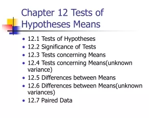
Chapter 14 Tests of Hypotheses Based on Count Data. 14.2 Tests concerning proportions (large samples) 14.3 Differences between proportions 14.4 The analysis of an r x c table. 14.2 Tests concerning proportions (large samples). np>5; n(1-p)>5 n independent trials; X=# of successes

E N D
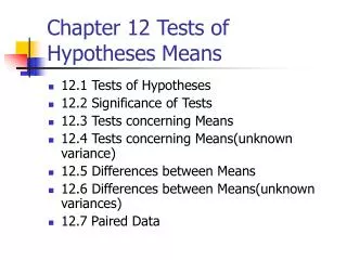
Chapter 14 Tests of Hypotheses Based on Count Data • 14.2 Tests concerning proportions (large samples) • 14.3 Differences between proportions • 14.4 The analysis of an r x c table
14.2 Tests concerning proportions (large samples) • np>5; n(1-p)>5 • n independent trials; • X=# of successes • p=probability of a success • Estimate:
Tests of Hypotheses • Null H0: p=p0 • Possible Alternatives: HA: p<p0 HA: p>p0 HA: pp0
Test Statistics • Under H0, p=p0, and • Statistic: is approximately standard normal under H0 . Reject H0 if z is too far from 0 in either direction.
Example 14.1 • H0: p=0.75 vs HA: p0.75 • =0.05 • n=300 • x=206 • Reject H0 if z<-1.96 or z>1.96
Observed z value • Conclusion: reject H0 since z<-1.96 • P(z<-2.5 or z>2.5)=0.0124<a reject H0.
Example 14.2 • Toss a coin 100 times and you get 45 heads • Estimate p=probability of getting a head Is the coin balanced one? a=0.05 Solution: H0: p=0.50 vs HA: p0.50
Enough Evidence to Reject H0? • Critical value z0.025=1.96 • Reject H0 if z>1.96 or z<-1.96 • Conclusion: accept H0
Truth = surgical biopsy Cancer Present Cancer Absent Total Result Positive 140 80 220 FNA status Results Negative 10 910 920 150 990 1140 Total Another example • The following table is for a certain screening test
Test to see if the sensitivity of the screening test is less than 97%. • Hypothesis • Test statistic
What is the conclusion? • Check p-value when z=-2.6325, p-value = 0.004 • Conclusion: we can reject the null hypothesis at level 0.05.
Truth = surgical biopsy Cancer Present Cancer Absent Total Result Positive 14 8 22 FNA status Results Negative 1 91 92 114 15 99 Total One word of caution about sample size: • If we decrease the sample size by a factor of 10,
And if we try to use the z-test, P-value is greater than 0.05 for sure (p=0.2026). So we cannot reach the same conclusion. And this is wrong!
So for test concerning proportions We want np>5; n(1-p)>5
14.3 Differences Between Proportions • Two drugs (two treatments) • p1 =percentage of patients recovered after taking drug 1 • p2 =percentage of patients recovered after taking drug 2 • Compare effectiveness of two drugs
Tests of Hypotheses • Null H0: p1=p2 (p1-p2 =0) • Possible Alternatives: HA: p1<p2 HA: p1>p2 HA: p1p2
Compare Two Proportions • Drug 1: n1 patients, x1 recovered • Drug 2: n2 patients, x2 recovered • Estimates: • Statistic for test: • If we did this study over and over and drew a histogram of the resulting values of , that histogram or distribution would have standard deviation
Estimating the Standard Error • Under H0, p1=p2=p. So • Estimate the common p by
Example 12.3 • Two sided test: • H0: p1=p2 vs HA: p1p2 • n1=80, x1=56 • n2=80, x2=38
Two Tailed Test • Observed z-value: • Critical value for two-tailed test: 1.96 • Conclusion: Reject H0 since |z|>1.96
P-value of the previous example • P-value=P(z<-2.88)+P(z>2.88)=2*0.004 • So not only we can reject H0 at 0.05 level, we can also reject at 0.01 level.
trt1 trt2 recover 56 38 94 66 24 42 Not recover 80 80 14.4 The analysis of an r x c table Recall Example 12.3 • Two sided test; H0: p1=p2 vs HA: p1p2 • n1=80, x1=56 n2=80, x2=38 We can put this into a 2x2 table and the question now becomes is there a relationship between treatment and outcome? We will come back to this example after we introduce 2x2 tables and chi-square test.
OUTCOME Survival for at least 28 days Death Total Propranolol 38 7 45 Treatment 29 17 46 Placebo 91 Total 67 24 2x2 Contingency Table • The table shows the data from a study of 91 patients who had a myocardial infarction (Snow 1965). One variable is treatment (propranolol versus a placebo), and the other is outcome (survival for at least 28 days versus death within 28 days).
Hypotheses for Two-way Tables • The hypotheses for two-way tables are very “broad stroke”. • The null hypothesis H0 is simply that there is no association between the row and column variable. • The alternative hypothesis Ha is that there is an association between the two variables. It doesn’t specify a particular direction and can’t really be described as one-sided or two-sided.
Hypothesis statement in Our Example • Null hypothesis: the method of treating the myocardial infarction patients did not influence the proportion of patients who survived for at least 28 days. • The alternative hypothesis is that the outcome (survival or death) depended on the treatment, meaning that the outcomes was the dependent variable and the treatment was the independent variable.
Calculation of Expected Cell Count • To test the null hypothesis, we compare the observed cell counts (or frequencies) to the expected cell counts (also called the expected frequencies) • The process of comparing the observed counts with the expected counts is called a goodness-of-fit test. (If the chi-square value is small, the fit is good and the null hypothesis is not rejected.)
OUTCOME OUTCOME Survival for at least 28 days Survival for at least 28 days Death Total Death Total 33.13 38 7 11.87 Propranolol Propranolol 45 45 Treatment Treatment 29 33.87 17 12.13 46 46 Placebo Placebo 91 91 Total Total 67 67 24 24 Observed cell counts Expected cell counts
The Chi-Square ( c2) Test Statistic • The chi-square statistic is a measure of how much the observed cell counts in a two-way table differ from the expected cell counts. It can be used for tables larger than 2 x 2, if the average of the expected cell counts is > 5 and the smallest expected cell count is > 1; and for 2 x 2 tables when all 4 expected cell counts are > 5. The formula is: • c2 = S(observed count – expected count)2/expected count • Degrees of freedom (df) = (r –1) x (c – 1) • Where “observed” is an observed sample count and “expected” is the computed expected cell count for the same cell, r is the number of rows, c is the number of columns, and the sum (S) is over all the r x c cells in the table (these do not include the total cells).
Example: Patient Compliance w/ Rx In a study of 100 patients with hypertension, 50 were randomly allocated to a group prescribed 10 mg lisinopril to be taken once daily, while the other 50 patients were prescribed 5 mg lisinopril to be taken twice daily. At the end of the 60 day study period the patients returned their remaining medication to the research pharmacy. The pharmacy then counted the remaining pills and classified each patient as < 95% or 95%+ compliant with their prescription. The two-way table for Compliance and Treatment was: Treatment Compliance10 mg Daily5 mg bidTotal 95%+ 46 40 86 < 95% 4 10 14 Total 50 50 100
The expected cell counts were: Treatment Compliance10 mg Daily5 mg bidTotal 95%+ 430 430 860 < 95% 70 70 140 Total 500 500 1000 Example: Patient Compliance w/ Rx Treatment Compliance10 mg Daily5 mg bidTotal 95%+ 460 400 860 < 95% 40 100 140 Total 500 500 1000 c2= 29.9, df = (2-1)*(2-1) = 1, P-value <0.001
The c2 and z Test Statistics The comparison of the proportions of “successes” in two populations leads to a 2 x 2 table, so the population proportions can be compared either using the c2 test or the two-sample z test . It really doesn’t matter, because they always give exactly the same result, because the c2 is equal to the square of the z statistic and the chi-square with one degree of freedom c2(1) critical values are equal to the squares of the corresponding z critical values. • A P-value for the 2 x 2 c2 can be found by calculating the square root of the chi-square, looking that up in Table for P(Z>z) and multiplying by 2, because the chi-square always tests the two-sided alternative. • For a 2 x 2 table with a one-sided alternative hypothesis the two-sample z statistic would need to be used. • To test more than two populations the chi-square must be used • The chi-square is the one most often seen in the literature
Summary: Computations for Two-way Tables • create the table, including observed cell counts, column and row totals. • Find the expected cell counts. • Determine if a c2 test is appropriate • Calculate the c2 statistic and number of degrees of freedom • Find the approximate P-value • use Table III chi-square table to find the approximate P-value • or use z-table and find the two-tailed p-value if it is 2 x 2. • Draw conclusions about the association between the row and column variables.
Yates Correction for Continuity • The chi-square test is based on the normal approximation of the binomial distribution (discrete), many statisticians believe a correction for continuity is needed. • It makes little difference if the numbers in the table are large, but in tables with small numbers it is worth doing. • It reduces the size of the chi-square value and so reduces the chance of finding a statistically significant difference, so that correction for continuity makes the test more conservative.
What do we do if the expected values in any of the cells in a 2x2 table is below 5? For example, a sample of teenagers might be divided into male and female on the one hand, and those that are and are not currently dieting on the other. We hypothesize, perhaps, that the proportion of dieting individuals is higher among the women than among the men, and we want to test whether any difference of proportions that we observe is significant. The data might look like this:
The question we ask about these data is: knowing that 10 of these 24 teenagers are dieters, what is the probability that these 10 dieters would be so unevenly distributed between the girls and the boys? If we were to choose 10 of the teenagers at random, what is the probability that 9 of them would be among the 12 girls, and only 1 from among the 12 boys? --Hypergeometric distribution! --Fisher’s exact test uses hypergeometric distribution to calculate the “exact” probability of obtaining such set of the values.
Fisher’s exact test Before we proceed with the Fisher test, we first introduce some notation. We represent the cells by the letters a, b, c and d, call the totals across rows and columns marginal totals, and represent the grand total by n. So the table now looks like this:
Fisher showed that the probability of obtaining any such set of values was given by the hypergeometric distribution:
men women total men women total dieting 1 9 10 dieting 0 10 10 not dieting 12 2 14 not dieting 11 3 14 totals 12 12 24 totals 12 12 24 More extreme than observed As extreme as observed In our example Recall that p-value is the probability of observing data as extreme or more extreme if the null hypothesis is true. So the p-value is this problem is 0.00137.
The fisher Exact Probability Test • Used when one or more of the expected counts in a contingency table is small (<2). • Fisher's Exact Test is based on exact probabilities from a specific distribution (the hypergeometric distribution). • There's really no lower bound on the amount of data that is needed for Fisher's Exact Test. You can use Fisher's Exact Test when one of the cells in your table has a zero in it. Fisher's Exact Test is also very useful for highly imbalanced tables. If one or two of the cells in a two by two table have numbers in the thousands and one or two of the other cells has numbers less than 5, you can still use Fisher's Exact Test. • Fisher's Exact Test has no formal test statistic and no critical value, and it only gives you a p-value.