Download
1 / 11
110 likes | 294 Views
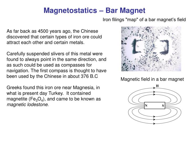
Magnetostatics – Bar Magnet. Iron filings "map" of a bar magnet’s field. As far back as 4500 years ago, the Chinese discovered that certain types of iron ore could attract each other and certain metals.

E N D
Magnetostatics – Bar Magnet Iron filings "map" of a bar magnet’s field As far back as 4500 years ago, the Chinese discovered that certain types of iron ore could attract each other and certain metals. Carefully suspended slivers of this metal were found to always point in the same direction, and as such could be used as compasses for navigation. The first compass is thought to have been used by the Chinese in about 376 B.C Greeks found this iron ore near Magnesia, in what is present day Turkey. It contained magnetite (Fe3O4), and came to be known as magnetic lodestone. Magnetic field in a bar magnet
Magnetostatics – Oersted’s Experiment A compass is an extremely simple device. A magnetic compass consists of a small, lightweight magnet balanced on a nearly frictionless pivot point. The magnet is generally called a needle. One end of the needle is often marked "N," for north, or colored in some way to indicate that it points toward north. On the surface, that's all there is to a compass In 1600, William Gilbert of England postulated that magnetic lodestones, or compasses, work because the earth is one big magnet. The magnetic field is generated by the spin of the molten inner core. The north end of a compass needle points to the geographic north pole, which corresponds to the earth’s south magnetic pole. The Earth can be thought of a gigantic bar magnet buried inside. In order for the north end of the compass to point toward the North Pole, you have to assume that the buried bar magnet has its south end at the North Pole. Magnetic Compass Magnetic Compass
Magnetostatics – Oersted’s Experiment Oersted’s experiment In 1820, Hans Christian Oersted (1777-1851) used a compass to show that current produces magnetic fields that loop around the conductor Magnetism and electricity were considered distinct phenomena until 1820 when Hans Christian Oersted conducted an experiment that showed a compass needle deflecting when in proximity to a current carrying wire. It was observed that moving away from the source of current, the field grows weaker. Oersted’s discovery released flood of study that culminated in Maxwell’s equations in 1865.
Magnetostatics – Biot-Savart’s Law Shortly following Oersted’s discovery that currents produce magnetic fields, Jean Baptiste Biot (1774-1862) and Felix Savart (1791-1841) arrived at a mathematical relation between the field and current. The Law of Biot-Savart is (A/m) To get the total field resulting from a current, you can sum the contributions from each segment by integrating (A/m) Note: The Biot-Savart law is analogous to the Coulomb’s law equation for the electric field resulting from a differential charge
Magnetostatics – An Infinite Line current Example 3.2: Consider an infinite length line along the z-axis conducting current I in the +az direction. We want to find the magnetic field everywhere. We first inspect the symmetry and see that the field will be independent of z and and only dependent on ρ. An infinite length line of current So we consider a point a distance r from the line along the ρ axis. The Biot-Savart Law IdL is simply Idzaz, and the vector from the source to the test point is The Biot-Savart Law becomes
Magnetostatics – An Infinite Line current Pulling the constants to the left of the integral and realizing that az x az = 0 and az x aρ = a, we have The integral can be evaluated using the formula given in Appendix D When the limit
Magnetostatics – An Infinite Line current An infinite length line of current Using We find the magnetic field intensity resulting from an infinite length line of current is Direction: The direction of the magnetic field can be found using the right hand rule. Magnitude: The magnitude of the magnetic field is inversely proportional to radial distance.
Magnetostatics – A Ring of Current Example 3.3: Let us now consider a ring of current with radius a lying in the x-y plane with a current I in the +az direction. The objective is to find an expression for the field at an arbitrary point a height h on the z-axis. The Biot-Savart Law The differential segment dL = ada The vector drawn from the source to the test point is Magnitude: Unit Vector: The biot-Savart Law can be written as
Magnetostatics – A Ring of Current We can further simplify this expression by considering the symmetry of the problem az components add A particular differential current element will give a field with an aρ component (from a x az) and an az component (from a x –aρ). Taking the field from a differential current element on the opposite side of the ring, it is apparent that the radial components cancel while the az components add. aρ Components Cancel H At h = 0, the center of the loop, this equation reduces to
Magnetostatics – A Solenoid A solenoid Solenoids are many turns of insulated wire coiled in the shape of a cylinder. Suppose the solenoid has a length h, a radius a, and is made up of N turns of current carrying wire. For tight wrapping, we can consider the solenoid to be made up of N loops of current. To find the magnetic field intensity from a single loop at a point P along the axis of the solenoid, from we have The differential amount of field resulting from a differential amount of current is given by The differential amount of current can be considered a function of the number of loops and the length of the solenoid as
Magnetostatics – A Solenoid Fixing the point P where the field is desired, z’ will range from –z to h-z, or This integral is found from Appendix D, leading to the solution At the very center of the solenoid (z = h/2), with the assumption that the length is considerably bigger than the loop radius (h >> a), the equation reduces to