Fast orbit bump magnet

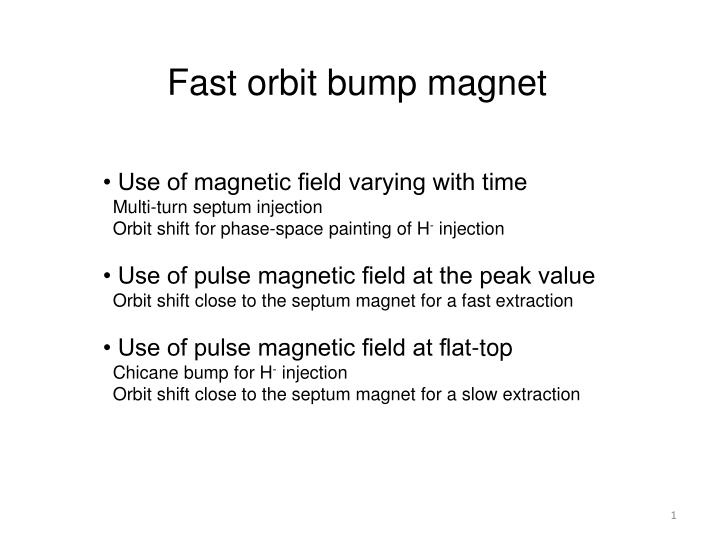
1. Fast orbit bump magnet • Use of magnetic field varying with time Multi-turn septum injection Orbit shift for phase-space painting of H- injection • Use of pulse magnetic field at the peak value Orbit shift close to the septum magnet for a fast extraction • Use of pulse magnetic field at flat-top Chicane bump for H- injection Orbit shift close to the septum magnet for a slow extraction

2. Orbit shift multi-turn injection by septum magnet Fig. 1 The principle of the multi turn injection

3. Use of decay field by critical damping The principle of the power supply circuit and its waveform are shown in Fig.2 The critical damping of the circuit is given as, The excitation current is given by next equation, Fig.2 Principle of the circuit Fast decay 1μs/div, 2V/div (50A/V) Slow decay Fig.3 Actual power supply circuit 1μs/div, 2V/div (50A/V)

4. Half sine wave by LC circuit for the use of peak value. Short time orbit-shift within the td Half sine Voltage recover Voltage recover

5. Combination of LC resonant circuit and LR damping circuit Principle of the circuit Actual power supply circuit 2μs/div, 5V/div (1kA/V) 5μs/div, 5V/div (1kA/V) 5μs/div, 5V/div (1kA/V) 5μs/div, 5V/div (1kA/V)

6. Fast orbit bump magnet for orbit shift multi-turn injection • Fast decay time (3~6 μs) • Ferrite is used for the core material. • Swing of the magnetic field is not allowed (for injection)

7. Characteristics of Ferrite (Fe2O3) Temperature characteristics Frequency characteristics

8. Longitudinal field distribution (measured value)

9. Excitation characteristics

10. Caution ! For “window frame” and “H-type core” • Shorted-magnetic circuit enclose the beam. • Magnetic resistance is very low. • Strong magnetic field is induced around bunched beams. • Open-magnetic circuit • Magnetic resistance is high. • Magnetic field induced around bunched beams is low. C-type is better !

11. Orbit bump magnet for Charge exchange injection Stripping Foil

12. Charge-exchange injection by chicane bump magnets

13. Parameters of H- injection bump magnet for the KEK Booster Cross section of the core with “end–slit”

14. Properties of core material (0.1 mm Thick silicon steel, Nihon Kinzoku ST-100)

15. B-H characteristics Iron loss

16. Excitation characteristics of the magnet

17. Longitudinal field distribution of chicane bump magnets Longitudinal field distribution of single bump magnet

18. Waveform of injection bump magnets(Use of magnetic field at the flat-top) 20μs/div, 2V/div, (1kA/V)

19. Pulse power supply by a pulse-forming-network (PFN) Ladder-type Line-type Ladder-type Rising phase of the wave form Falling phase of the wave form

20. Pulse forming network for chicane bump magnets (Using flattop field for injection)

21. PFN voltage, Magnet current and Magnet voltage 1ms/div, 5V/div (1kV/V) 50μs/div, 2V/div (1kA/V) 50μs/div, 0.5V/div

22. Fundamentals of Transmission Line Theory “Exact transitional solution” Let’s consider the part of transmission line as, x x + Δx On the one side line, partial resistance and inductance per unit length are (R/2) and (L/2) respectively. By the go and the return the values become R and L. The capacitance and conductance between two lines are defined as C and G respectively.

23. Equations for v and i are given as, finite difference equation. (1) Divide both sides by Δx and in the limit of Δx→0, we can get next differential equations. (2) These simultaneous partial differential equations are known as “Telegraphy equation”

24. In the case of lossless transmission line,i.e. R = G = 0. The telegraphy equation becomes Here, (3) We can get wave equations. Here (4) The solution of Eq.(4) is given as, (5) v and i must satisfy the Eq.(3), we can get next solution for i, (6)

25. Eq.(5) and (6) satisfies wave equation. Final solution can be obtained by initial condition of “t” and boundary condition of “x”. Here we define the initial value of “v” and “t“ as v(x,0) and i(x,0) respectively. Then we perform Laplace transformation for Eq.(3) and (4). (7) (8) For the case of initial values are zero. (or v(x,0)=0 and i(x,0)=0 ) (9) Eq.(9) is equivalent to Eq.(5) and Eq.(6).

26. In the Eq.(9), V1and V2 are decided by boundary condition of the x. When a voltage source e(t) is connected at x=0, The Laplace transformation of e(t) is written as, L{e(t)}=E(s). For a current source i(t), it is also as, L{i(t)}=I(s). Those are, at x=0, the voltage source e(t) is connected; V(0,s)=E(s) at x=0, the current source i(t) is connected; I(0,s)=I(s) The length of the transmission line is “ l ” at x=l, the terminal is shorten; V(l,s)=0 at x=l, the terminal is open; I(l,s)=0 at x=l, Z(s) is connected; V(l,s) / I(l,s)=Z(s) For example, a voltage source e(t) with internal impedance Z0(s) are connected at x=0 as shown in Fig. The conditional equation is,

27. Terminal is shorted-circuit as in Fig. A electromotive force is connected at x=0, and the terminal at x=l is shortened. The boundary condition is, at x=0 ; V(0,s)=E(s) at x=l ; V(l,s)=0 From Eq.(9) first, (10) We can solve Eq.(10) for V1 and V2, and substitute them to Eq.(9), the Laplace transform of the voltage v and current I is calculated as, (11) (12) Here, (characteristic impedance)

28. After rearrangement of the Eq.(11), then expand it in a series, (13) By the same procedure, we can get the I(x,s) as, (14) By inverse Laplace transformation (15)

29. Terminal is shorted-circuit “For intuitive understanding” Response for step voltage function (Opposite phase reflection)

30. Terminal is shorted-circuit Response for step current function (Same phase reflection)

31. Terminal is open circuit as in Fig. A electromotive force is connected at x=0, and the terminal at x=l is opened. The boundary condition is, (16) We can solve Eq.(16) for V1 and V2, and substitute them to Eq.(9), the Laplace transform of the voltage v and current I is calculated. Then expand it in a series and next by inverse Laplace transformation, we can get v(x,t) and i(x,t) as, (17)

32. Terminal is open-circuit Response for step voltage function (Same phase reflection)

33. Terminal is open-circuit Response for step current function (Opposite phase reflection)

34. Z(s) is connected to the terminal. The boundary condition is, Here, we set Z(s)=R for the simplicity. W is the characteristic impedance.

35. “reflection coefficient” For Z = 0, the terminal is shorted circuit. r = -1 For Z = ∞, the terminal is open circuit. r = 1 “Intuitive understanding” Same phase reflection Opposite phase reflection Sum of the “go” and “return” waves Sum of the “go” and “return” waves

36. Combined bump-septum magnet system for negative-positive ion injection

37. Structure of combined bump-septum magnet

38. Magnetic field of the combined bump-septum magnet

39. How to get a steep septum magnetic field

40. Measured value of magnetic field

41. Change of the bump magnet field by exciting the septum magnet

42. Figure of combined bump-septum magnet

43. Figure of combined bump-septum magnet

44. Mechanical structure of the combined bump-septum magnet

45. Magnetic field distribution of “Normal septum”and “Combined septum”

46. Comparison of “Normal septum”and “Combined septum”

47. Power supply system for the H-injection bump magnets

48. Power supply system for the combined bump-septum magnet system

49. Current waveform of the combined septum conductor (Superimpose rectangular waves) 20μs/div, 5V/div (1kA/V) (a); Septum current (b); Main bump current