Download
1 / 18
180 likes | 391 Views
Route Choice. CEE 320 Steve Muench. Outline. General HPF Functional Forms Basic Assumptions Route Choice Theories User Equilibrium System Optimization Comparison. Route Choice. Equilibrium problem for alternate routes Requires relationship between: Travel time (TT) Traffic flow (TF)

E N D
Route Choice CEE 320Steve Muench
Outline • General • HPF Functional Forms • Basic Assumptions • Route Choice Theories • User Equilibrium • System Optimization • Comparison
Route Choice • Equilibrium problem for alternate routes • Requires relationship between: • Travel time (TT) • Traffic flow (TF) • Highway Performance Function (HPF) • Common term for this relationship
HPF Functional Forms Common Non-linear HPF Linear Travel Time FreeFlow Non-Linear from the Bureau of Public Roads (BPR) Capacity Traffic Flow (veh/hr)
Basic Assumptions • Travelers select routes on the basis of route travel times only • People select the path with the shortest TT • Premise: TT is the major criterion, quality factors such as “scenery” do not count • Generally, this is reasonable • Travelers know travel times on all available routes between their origin and destination • Strong assumption: Travelers may not use all available routes, and may base TTs on perception • Some studies say perception bias is small
Theory of User Equilibrium Travelers will select a route so as to minimize their personal travel time between their origin and destination. User equilibrium (UE) is said to exist when travelers at the individual level cannot unilaterally improve their travel times by changing routes. Wadrop definition: A.K.A. Wardrop’s 1st principle “The travel time between a specified origin & destination on all used routes is equal, and less than or equal to the travel time that would be experienced by a traveler on any unused route”
Formulating the UE Problem Finding the set of flows that equates TTs on all used routes can be cumbersome. Alternatively, one can minimize the following function:
Example (UE) • Two routes connect a city and a suburb. During the peak-hour morning commute, a total of 4,500 vehicles travel from the suburb to the city. Route 1 has a 60-mph speed limit and is 6 miles long. Route 2 is half as long with a 45-mph speed limit. The HPFs for the route 1 & 2 are as follows: • Route 1 HPF increases at the rate of 4 minutes for every additional 1,000 vehicles per hour. • Route 2 HPF increases as the square of volume of vehicles in thousands per hour. Compute UE travel times on the two routes. Route 1 Suburb City Route 2
Example: Solution • Determine HPFs • Route 1 free-flow TT is 6 minutes, since at 60 mph, 1 mile takes 1 minute. • Route 2 free-flow TT is 4 minutes, since at 45 mph, 1 mile takes 4/3 minutes. • HPF1 = 6 + 4x1 • HPF2 = 4 + x22 • Flow constraint: x1 + x2 = 4.5 • Route use check (will both routes be used?) • All or nothing assignment on Route 1 • All or nothing assignment on Route 2 • Therefore, both routes will be used If all the traffic is on Route 1 then Route 2 is the desirable choice If all the traffic is on Route 2 then Route 1 is the desirable choice
Example: Solution • Equate TTs • Apply Wardrop’s 1st principle requirements. All routes used will have equal times, and ≤ those on unused routes. Hence, if flows are distributed between Route1 and Route 2, then both must be used on travel time equivalency bases.
Example: Mathematical Solution Same equation as before
Theory of System-Optimal Route Choice Wardrop’s Second Principle: Preferred routes are those, which minimize total system travel time. With System-Optimal (SO) route choices, no traveler can switch to a different route without increasing total system travel time. Travelers can switch to routes decreasing their TTs but only if System-Optimal flows are maintained. Realistically, travelers will likely switch to non-System-Optimal routes to improve their own TTs.
Formulating the SO Problem Finding the set of flows that minimizes the following function:
Example (SO) • Two routes connect a city and a suburb. During the peak-hour morning commute, a total of 4,500 vehicles travel from the suburb to the city. Route 1 has a 60-mph speed limit and is 6 miles long. Route 2 is half as long with a 45-mph speed limit. The HPFs for the route 1 & 2 are as follows: • Route 1 HPF increases at the rate of 4 minutes for every additional 1,000 vehicles per hour. • Route 2 HPF increases as the square of volume of vehicles in thousands per hour. Compute UE travel times on the two routes. Route 1 Suburb City Route 2
Example: Solution • Determine HPFs as before • HPF1 = 6 + 4x1 • HPF2 = 4 + x22 • Flow constraint: x1 + x2 = 4.5 • Formulate the SO equation • Use the flow constraint(s) to get the equation into one variable
Example: Solution • Minimize the SO function • Solve the minimized function • Find the total vehicular delay
User equilibrium t1 = 12.4 minutes t2 = 12.4 minutes x1 = 1,600 vehicles x2 = 2,900 vehicles tixi = 55,800 veh-min System optimization t1 = 14.3 minutes t2 = 10.08 minutes x1 = 2,033 vehicles x2 = 2,467 vehicles tixi = 53,592 veh-min Compare UE and SO Solutions Route 1 Suburb City Route 2
Primary Reference • Mannering, F.L.; Kilareski, W.P. and Washburn, S.S. (2005). Principles of Highway Engineering and Traffic Analysis, Third Edition. Chapter 8