Download
1 / 19
220 likes | 440 Views
PID CONTROLLER. Introduction . Pengendali otomatis membandingkan nilai sebenarnya dari keluaran sistem dengan masukannya, menentukan penyimpangan dan menghasilkan sinyal kendali yang akan mengurangi penyimpangan sehingga menjadi nol atau sekecil mungkin.

E N D
Introduction Pengendali otomatis membandingkan nilai sebenarnya dari keluaran sistem dengan masukannya, menentukan penyimpangan dan menghasilkan sinyal kendali yang akan mengurangi penyimpangan sehingga menjadi nol atau sekecil mungkin. Pengendali proportional, integral dan derivative (PID) sangat populer di industri karena sederhana dalam desainnya dan sudah teruji kehandalannya.
The three-term controller • Transfer function dari pengendali PID adalah sebagai berikut: • Kp = Proportional gain • KI = Integral gain • Kd = Derivative gain • Dari blok diagram sistem close loop diatas, sinyal error (e) akan dikirim ke PID controller, selanjutnya PID controller akan menghitung dan mengeluarkan sinyal control law (u) sebesar: • Sinyal (u) akan dikirim ke plant sehingga output baru (Y) akan diperoleh.
The characteristics of P, I, and D controllers • Proportional controller Kp berdampak: mengurangi rise time, mengurangi tapi tidak bisa menghilangkan steady state error. • Integral controller Ki berdampak: menghilangkan steady state error namun membuat transient respon-nya jelek. • Derivative controller Kd berdampak: meningkatkan stabilitas sistem, mengurangi overshoot dan memperbaiki transient response.
Example Problem Persamaan differensial sistem disamping adalah: Dengan transformasi Laplace didapat: Transfer function dari sistem ini adlah: Misalnya diambil data: M = 1kg b = 10 N.s/m k = 20 N/m F(s) = 1
Memasukkan data diatas kedalam transfer function diperoleh: • Kita akan memdesain PID controller dengan design criteria sbb: • Fast rise time • Minimum overshoot • No steady-state error
Open-loop step response Matlab program: num=1; den=[1 10 20]; plant=tf(num,den); step(plant) steady-state error of 0.95 rise time is about one second and the settling time is about 1.5 seconds. Let's design a controller that will reduce the rise time, reduce the settling time, and eliminates the steady-state error.
Proportional control The closed-loop transfer function of the above system with a proportional controller is: Misalnya Kp=300: Kp=300; contr=Kp; sys_cl=feedback(contr*plant,1); t=0:0.01:2; step(sys_cl,t) The above plot shows that the proportional controller reduced both the rise time and the steady-state error, increased the overshoot, and decreased the settling time by small amount.
Proportional-Derivative control The closed-loop transfer function of the given system with a PD controller is: Let Kp equal 300 as before and let Kd equal 10. Kp=300; Kd=10; contr=tf([Kd Kp],1); sys_cl=feedback(contr*plant,1); t=0:0.01:2; step(sys_cl,t) This plot shows that the derivative controller reduced both the overshoot and the settling time, and had a small effect on the rise time and the steady-state error.
Proportional-Integral control For the given system, the closed-loop transfer function with a PI control is: Let's reduce the Kp to 30, and let Ki equal 70. Kp=30; Ki=70; contr=tf([Kp Ki],[1 0]); sys_cl=feedback(contr*plant,1); t=0:0.01:2; step(sys_cl,t) The above response shows that the integral controller eliminated the steady-state error.
Proportional-Integral-Derivative control The closed-loop transfer function of the given system with a PID controller is: After several trial and error runs, the gains Kp=350, Ki=300, and Kd=50 provided the desired response. Kp=350; Ki=300; Kd=50; contr=tf([Kd Kp Ki],[1 0]); sys_cl=feedback(contr*plant,1); t=0:0.01:2; step(sys_cl,t) Now, we have obtained a closed-loop system with no overshoot, fast rise time, and no steady-state error.
General tips for designing a PID controller • Obtain an open-loop response and determine what needs to be improved • Add a proportional control to improve the rise time • Add a derivative control to improve the overshoot • Add an integral control to eliminate the steady-state error • Adjust each of Kp, Ki, and Kd until you obtain a desired overall response. You can always refer to the table shown in this "PID Tutorial" page to find out which controller controls what characteristics.
Example: PID Design method for the Pitch Controller EOM of an aircraft can be decoupled and linearized into the longitudinal and lateral equations. Pitch control is a longitudinal problem, and in this example, we will design an autopilot that controls the pitch of an aircraft. The longitudinal equations of motion of an aircraft can be written as:
Transfer function model • Let's plug in some numerical values to simplify the modeling equations (1) shown above. • These values are taken from the data from one of Boeing's commercial aircraft. • The Laplace transform of the above equations are shown below. • After few steps of algebra, you should obtain the following transfer function.
Design requirements • Overshoot: Less than 10% • Rise time: Less than 2 seconds • Settling time: Less than 10 seconds • Steady-state error: Less than 2%
MATLAB representation and open-loop response Let the input (delta e) be 0.2 rad (11 degrees). de=0.2; num=[1.151 0.1774]; den=[1 0.739 0.921 0]; pitch=tf(num,den); step(de*pitch)axis([0 15 0 0.8]) From the plot, we see that the open-loop response does not satisfy the design criteria at all. In fact the open-loop response is unstable.
Proportional control The closed-loop transfer function of the system as: Kp=[1]; num=[1.151 0.1774]; den=[1 0.739 0.921 0]; pitch=tf(num,den); contr=tf(Kp,1); sys_cl=feedback(contr*pitch,1); let the proportional gain (Kp) equal 2 de=0.2; Kp=2; sys_cl=feedback(Kp*pitch,1); t=0:0.01:30; step(de*sys_cl,t) As you see, both the overshoot and the settling time need some improvement.
PD control The closed-loop transfer function of the system with a PD controller is: Let a proportional gain (Kp) of 9 and a derivative gain (Kd) of 4, de=0.2; Kp=9; Kd=4; contr=tf([Kd Kp],1); sys_cl=feedback(contr*pitch,1); t=0:0.01:10; step(de*sys_cl,t) This step response shows the rise time of less than 2 seconds, the overshoot of less than 10%, the settling time of less than 10 seconds, and the steady-state error of less than 2%. All design requirements are satisfied.
PID control Let the proportional gain (Kp) of 2, the integral gain (Ki) of 4, and the derivative gain (Kd) of 3: de=0.2; Kp=2; Kd=3; Ki=4; num=[1.151 0.1774]; den=[1 0.739 0.921 0]; pitch=tf(num,den); contr=tf([Kd Kp Ki],[1 0]); sys_cl=feedback(contr*pitch,1); t=0:0.01:10; step(de*sys_cl,t)