Scientific Methods 1

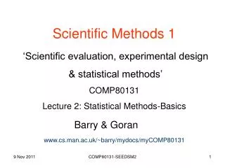
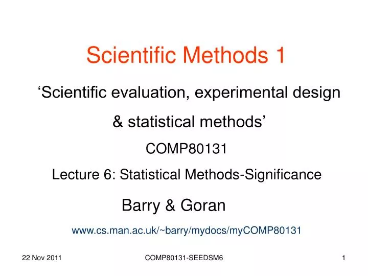
Scientific Methods 1 ‘Scientific evaluation, experimental design & statistical methods’ COMP80131 Lecture 6: Statistical Methods-Significance Barry & Goran www.cs.man.ac.uk/~barry/mydocs/myCOMP80131 COMP80131-SEEDSM6

pdf(x) 1 x a b 1 pdf(x) m a b x m- m+ Continuous random processes • Characterised by probability density functions (pdf) Uniform pdf: Prob of the random variable x lying between a and b is: Gaussian (Normal) pdf with mean m & std dev . 95.5% for m  299.7% for m  3 68% COMP80131-SEEDSM6

pdf & Histograms • Ru = rand(10000,1); %10000 unif samples • hist(Ru,20); • Rg=randn(10000,1); %Gaussian with m=0, std=1 • hist(Rg,20); COMP80131-SEEDSM6

Convert histogram to estimate of pdf • Divide each column by number of samples • Then multiply by number width of bins. • For better approximation, increase number of bins COMP80131-SEEDSM6

MATLAB illustration Rg = randn(100000,1); %10000 Gaussians with m=0, std=1 widthBin = 0.2; X = -4 : widthBin : 4 ; H = hist(Rg,X); % Histogram with bins centred on elements of X figure(2); bar(X,(H/100000)/widthBin); ylabel('pdf estimate'); Histogram as pdf estimate. COMP80131-SEEDSM6

Gaussian (normal) pdf • Measurements {xi} of many naturally occurring phenomena tend to be normally distributed with some mean m & std . • Let zi = (xi - m)/, • Then {zi} will have a standard normal pdf with mean = 0 & std = 1. COMP80131-SEEDSM6

0.4 0.35 0.3 Gaussian pdf 0.25 0.2 0.15 0.1 0.05 0 -4 -3 -2 -1 0 1 2 3 4 x Plot true standard normal pdf Mean=0; Std=1; K = 1/( Std*sqrt(2*pi) ); X = -4*Std : widthBin : 4*Std ; for I=1:length(X); G(I) = K * exp(-(X(I)-Mean)^2 / (2*Std^2) ); end; figure(4); plot(X,G); ylabel('pdf'); COMP80131-SEEDSM6

Plot Gaussian cdf X=-4:0.1:4; C = normcdf(X,0,1); figure(1); plot(X,C); grid on; xlabel('x'); ylabel('prob that var < x'); Cumulative density function (cdf) Probability of Gaussian variable (m=0 std=1)being < x. No formula for this. Use MATLAB function: normcdf(X,m,std) COMP80131-SEEDSM6

1 0.9 0.8 0.7 0.6 prob that var > x 0.5 0.4 0.3 0.2 0.1 0 -4 -3 -2 -1 0 1 2 3 4 x Complementary Gaussian cdf This is just 1 – normcdf(x,m,) It is prob of Gaussian random variable (mean= m, std=) being > x. COMP80131-SEEDSM6

Complementary error function • Some call the complementary Gaussian cdf (m=0, =1) the ‘complementary error function’ Q(z) • But ‘erfc’ is also called this. • Q(z) = comp-Gaussian cdf= 0.5  erfc(-z/2). • Used to rely on tables & graphs of Q(z). • When m0 & 1, use Q((z-m)/) COMP80131-SEEDSM6

COMP80131-SEEDSM6

D E Use of ‘normcdf’ function Prob of random var being between D & E is: COMP80131-SEEDSM6

D Tail of distribution Prob of random variable being greater than D is: COMP80131-SEEDSM6

Voltage +1 +1/2 t An Engineering Question • Rectangular 1v & 0v pulses used to transmit a binary signal. • Affected by additive white Gaussian noise (AWGN). • Mean of noise =0 & power (variance) 2 = 0.01. • Estimate the bit-error probability. • Bit-error may occur if noise adds voltage > 0.5v to 0 v or < -0.5 v to 1v. • Assume same no. of 1’s & 0’s COMP80131-SEEDSM6

Solution prob(error) = prob(noise > 0.5) when bit =0 + prob(noise < -0.5) when bit =1 = 0.5  prob(noise > 0.5) +0.5  prob(noise < -0.5) = prob(noise > 0.5) because of symmetry = 1 - normcdf(0.5, 0, 0.1) = 2.910-7 Or, using graph Q(z/) on next page, prob(error) = Q(0.5/) = Q(0.5/0.1) = Q(5)  310-7 COMP80131-SEEDSM6

/ Q(z/) z/ COMP80131-SEEDSM6

Back to sampling • A population has true mean  & std . • Take a sample of N measurements from it – say N=50 • Calculate sample-mean m1 & std s1. • If population is Gaussian, pdf of m1 will be Gaussian with mean =  & std = s1 =  / N. • Can confirm by taking more samples to obtain sample-means & stds: m1, m2, …, mM & s1, s2, …, sM • Estimate mean & std of sample-means • Also mean & std of sample-variances (later) COMP80131-SEEDSM6

Significance testing • Assume pop-mean  (‘mu’)may change with pop-std fixed at . • Assume know pop-std  & that it will not change. • We can only take one sample of 50 values. • Calculate m1 to decide whether pop-mean has changed. • Null Hypothesis – it has not changed. new pop-mean New =  • If Null Hyp is true, pdf of sample-mean is on next slide: COMP80131-SEEDSM6

Concept of a ‘null-hypothesis’ • A null-hypothesis is an assumption that is made and then tested by a set of experiments designed to reveal that it is likely to be false, if it is false. • Testing is done by considering how probable the results are, assuming the null hypothesis is true. • If the results appear very improbable the researcher may conclude that the null-hypothesis is likely to be false. • This is usually the outcome the researcher hopes for when he or she is trying to prove that a new technique is likely to have some value. COMP80131-SEEDSM6

pdf of sample-mean m1 0.4 0.35 0.3 Gaussian pdf 0.25 s1 = /50 0.2 0.15 0.1 0.05 0 -2s1 -s1  +s1 +2 +4s1 m1 Assume value we got was m1 =  + 2.5s1. How unlikely if Null Hyp is true? COMP80131-SEEDSM6

p-value • “Probability of obtaining a test result at least as extreme as the one that was actually observed, assuming that the null hypothesis is true”. • Reject the null hypothesis if the p-value is less than some value α (significance level) which is often 0.05 or 0.01. • When the null-hypothesis is rejected, the result is said to be statistically significant. • Here p-value is 1 - normcdf(m1, , s1) …with s1= /N • = 1-normcdf(+2.5s1, , s1) • = 1- normcdf(2.5 ,0, 1) = 0.0062 • Much less than 0.01 so reject NH at 1% confidence level. • Conclude that mean has changed. COMP80131-SEEDSM6

Our 2 assumptions • That was easy because we made 2 assumptions: population is Gaussian & pop-std is known to us. • Now need to eliminate these 2 assumptions. • We have some help from the Central Limit Theorem: COMP80131-SEEDSM6

Central Limit Theorem • If samples of size N are ‘randomly’ chosen from a pop with mean  & std , the pdf of their mean, m1 say, approaches a Normal (Gaussian) pdf with mean  & std /N as N is made larger & larger. • Regardless of whether the population is Gaussian or not! • Previous example can be made to work for non-Gaussian pop provided N is ‘large enough’. • More on this next week. COMP80131-SEEDSM6

Another example • Assume we wish to find out if a proposed technique designed to benefit users of a system is likely to have any value. • Divide the users into two groups and offer the proposed technique to one group and something different to the other group. • The null-hypothesis would be that the proposed technique offers no measurable advantage over the other techniques. COMP80131-SEEDSM6

The testing • This would be carried out by looking for differences between the sets of results obtained for each of the two groups. • Careful experimental design will try to eliminate differences not caused by the techniques being compared. • Must take a large number of users in each group & randomize the way the users are assigned to groups. • Once other differences have been eliminated as far as possible, any remaining difference will hopefully be indicative of the effectiveness of the techniques being investigated. • The vital question is whether they are likely to be due to the advantages of the new technique, or the inevitable random variations that arise from the other factors. • Are the differences statistically significant? • Can employ a statistical significance to find out. COMP80131-SEEDSM6

Failure of the experiment • If the results are not found to look improbable under the null-hypothesis, i.e. if the differences between the two groups are not statistically significant, then no conclusion can be made. • The null-hypothesis could be true, or it could still be false. • It would be a mistake to conclude that the ‘null-hypothesis’ has been proved likely to be true in this circumstance. • It is quite possible that the results of the experiment give insufficient evidence to make any conclusions at all. COMP80131-SEEDSM6

Question: fair coin test Checking whether a coin is fair Suppose we obtain heads 14 times out of 20 flips. The p-value for this test result would be the probability of a fair coin landing on heads at least 14 times out of 20 flips. From binomial distribution formula( Lecture 4), this is: (20C14 + 20C15+20C16+20C17+20C18+20C19+20C20) / 220 = 0.058 This is probability that a fair coin would give a result as extreme or more extreme than 14 heads out of 20. COMP80131-SEEDSM6

Significance test for fair coin question • Reject null-hypothesis if p-value  α . • If α= 0.05, rejection of null-hypothesis is: “at the 5% (significance) level”. • Probability of wrongly rejecting null-hypothesis (Type 1 error) will be equal to α. • This is considered sufficiently low. • In this case, p-value > 0.05, therefore observation is consistent with null-hypothesis & we cannot reject it. • Cannot conclude that coin is likely to be unfair. • But we have NOT proved that coin is likely to be fair. • 14 heads out of 20 flips can be ascribed to chance alone • It falls within the range of what could happen 95% of the time with a fair coin. COMP80131-SEEDSM6

Questions from Lecture 2 • Analyse the ficticious exam results & comment on features. • Compute means, stds & vars for each subject & histograms for the distributions. • Make observations about performance in each subject & overall • Do marks support the hypothesis that people good at Music are also good at Maths? • Do they support the hypothesis that people good at English are also good at French? • Do they support the hypothesis that people good at Art are also good at Maths? • If you have access to only 50 rows of this data, investigate the same hypotheses • What conclusions could you draw, and with what degree of certainty? COMP80131-SEEDSM6

Questions from L4 • A patent goes to a doctor with a bad cough & a fever. The doctor needs to decide whether he has ‘swine flu’. Let statement S = ‘has bad cough and fever’ & statement F = ‘has swine flu’. The doctor consults his medical books and finds that about 40% of patients with swine-flu have these same symptoms. Assuming that, currently, about 1% of the population is suffering from swine-flu and that currently about 5% have bad cough and fever (due to many possible causes including swine-flu), we can apply Bayes theorem to estimate the probability of this particular patient having swine-flu. • A doctor in another country knows form his text-books that for 40% of patients with swine-flu, the statement S, ‘has bad cough and fever’ is true. He sees many patients and comes to believe that the probability that a patient with ‘bad cough and fever’ actually has swine-flu is about 0.1 or 10%. If there were reason to believe that, currently, about 1% of the population have a bad cough and fever, what percentage of the population is likely to be suffering from swine-flu? COMP80131-SEEDSM6

Scientific Methods 1