Graph Partitioning

1. Graph Partitioning James Demmel www.cs.berkeley.edu/~demmel/cs170_Spr10

2. Outline of Graph Partitioning Lecture • Review definition of Graph Partitioning problem • Overview of heuristics • Partitioning with Nodal Coordinates • Ex: node at point in (x,y) or (x,y,z) space • Partitioning without Nodal Coordinates • Ex: In model of WWW, nodes are web pages • Multilevel Acceleration • BIG IDEA, appears often in computing • Available software • Comparison of Methods and Applications

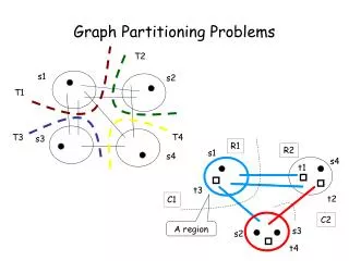
3. Definition of Graph Partitioning • Given a graph G = (N, E, WN, WE) • N = nodes (or vertices), • WN = node weights • E = edges • WE = edge weights • Ex: N = {tasks}, WN = {task costs}, edge (j,k) in E means task j sends WE(j,k) words to task k • Goal: Choose a partition N = N1 U N2 U … U NP such that • The sum of the node weights in each Nj is “about the same” • The sum of all edge weights of edges connecting all different pairs Nj and Nk is minimized • “Balance the work load, while minimizing communication” • Special case of N = N1 U N2: Graph Bisection 2 (2) 1 3 (1) 4 1 (2) 2 4 (3) 3 1 2 2 5 (1) 8 (1) 1 6 5 6 (2) 7 (3)

4. Definition of Graph Partitioning • Given a graph G = (N, E, WN, WE) • N = nodes (or vertices), • WN = node weights • E = edges • WE = edge weights • Ex: N = {tasks}, WN = {task costs}, edge (j,k) in E means task j sends WE(j,k) words to task k • Goal: Choose a partition N = N1 U N2 U … U NP such that • The sum of the node weights in each Nj is “about the same” • The sum of all edge weights of edges connecting all different pairs Nj and Nk is minimized (shown in black) • “Balance the work load, while minimizing communication.” • Special case of N = N1 U N2: Graph Bisection 2 (2) 1 3 (1) 4 1 (2) 2 4 (3) 3 1 2 2 5 (1) 8 (1) 1 6 5 6 (2) 7 (3)

5. Some Applications • Telephone network design • Original application, algorithm due to Kernighan • Load Balancing while Minimizing Communication • Operations on Sparse Matrices • Analogous to graphs with |E| << |N|2 • Important kernel in scientific computing • VLSI Layout • N = {units on chip}, E = {wires}, WE(j,k) = wire length • Data mining and clustering • Physical Mapping of DNA • Image Segmentation

6. A Sparse Matrix/Graph You Use Every Day

7. Cost of Graph Partitioning • Many possible partitionings to search • Just to divide n = |N| vertices into 2 equal subsets there are: n choose n/2 = n!/((n/2)!)2 ~ sqrt(2/(np))*2npossibilities • Choosing optimal partitioning is NP-complete • We need good heuristics • Goal: O(|E|)

8. Outline of Graph Partitioning Lecture • Review definition of Graph Partitioning problem • Overview of heuristics • Partitioning with Nodal Coordinates • Ex: node at point in (x,y) or (x,y,z) space • Partitioning without Nodal Coordinates • Ex: In model of WWW, nodes are web pages • Multilevel Acceleration • BIG IDEA, appears often in computing • Available software • Comparison of Methods and Applications

9. First Heuristic: Repeated Graph Bisection • To partition N into 2k parts • bisect graph recursively k times • Henceforth discuss mostly graph bisection

10. Overview of Bisection Heuristics • Partitioning with Nodal Coordinates • Each node has x,y coordinates and (mostly) connected just to nearest neighbors in space  partition space • Partitioning without Nodal Coordinates • E.g., Sparse matrix of Web documents • A(j,k) = # times keyword j appears in URL k • Multilevel acceleration (BIG IDEA) • Approximate problem by “coarse graph,” do so recursively

11. Outline of Graph Partitioning Lecture • Review definition of Graph Partitioning problem • Overview of heuristics • Partitioning with Nodal Coordinates • Ex: In finite element models, node at point in (x,y) or (x,y,z) space • Partitioning without Nodal Coordinates • Ex: In model of WWW, nodes are web pages • Multilevel Acceleration • BIG IDEA, appears often in scientific computing • Available software • Comparison of Methods and Applications

12. Coordinate-Free: Kernighan/Lin • Take a initial partition and iteratively improve it • Kernighan/Lin (1970), cost = O(|N|3) but easy to understand • Fiduccia/Mattheyses (1982), cost = O(|E|), much better, but more complicated • Given G = (N,E,WE) and a partitioning N = A U B, where |A| = |B| • T = cost(A,B) = S {W(e) where e connects nodes in A and B} • Find subsets X  A and Y  B with |X| = |Y| • Consider swapping X and Y if it decreases cost: • newA = (A – X) U Y and newB = (B – Y) U X • newT = cost(newA , newB) < T = cost(A,B) • Need to compute newT efficiently for many possible X and Y, choose smallest (best)

13. Coordinate-Free: Kernighan/Lin • Def: Suppose N = A U B, a  A, b B. Then gain(a,b) = gain from swapping a and b = sum of edge weights crossing between A and B - sum of edge weights crossing between A-{a}U{b} and B-{b}U{a} • If gain(a,b) > 0, swapping a and b helps, else not

14. Coordinate-Free: Kernighan/Lin Repeat … greedily try n/2 pairs (a,b) to swap, where aA, bB, n = |N| unmark all vertices while there are unmarked vertices pick unmarked pair (a,b) maximizing gain(a,b) … note that gain(a,b) might be negative mark a and b update all values of gain(x,y) for all unmarked x, y as though we had swapped a and b (but don’t swap them!) end while … at this point we have a sequence of possible pairs to swap … (a1,b1), (a2,b2),….,(an/2,bn/2), with gain1, gain2,…,gainn/2 … Suppose we swap X = {a1,…,am} and Y = {b1,…,bm}, … then the total gain would be Gain(m) = gain1 + gain2 + … + gainm Choose m to maximize Gain(m) If Gain(m) > 0, swap X = {a1,…,am} and Y = {b1,…,bm} until Gain(m)  0 … no improvement possible

15. Comments on Kernighan/Lin Algorithm • Some gain(k) may be negative, but if later gains are large, then final Gain(m) may be positive • can escape “local minima” where switching no pair helps • How many times do we Repeat? • K/L tested on very small graphs (|N|<=360) and got convergence after 2-4 sweeps • For random graphs (of theoretical interest) the probability of convergence in one step appears to drop like 2-|N|/30 • Better: multilevel approach (next)

16. Outline of Graph Partitioning Lectures • Review definition of Graph Partitioning problem • Overview of heuristics • Partitioning with Nodal Coordinates • Ex: node at point in (x,y) or (x,y,z) space • Partitioning without Nodal Coordinates • Ex: In model of WWW, nodes are web pages • Multilevel Acceleration • BIG IDEA, appears often in computing • Available software • Comparison of Methods and Applications

17. Introduction to Multilevel Partitioning • If we want to partition G(N,E), but it is too big to do efficiently, what can we do? • 1) Replace G(N,E) by a coarse approximation Gc(Nc,Ec), and partition Gc instead • 2) Use partition of Gc to get a rough partitioning of G, and then iteratively improve it • What if Gc still too big? • Apply same idea recursively

18. Multilevel Partitioning - High Level Algorithm (A,B ) = Multilevel_Partition( N, E ) … recursive partitioning routine returns A and B where N = A U B if |N| is small (1) Partition G = (N,E) directly to get N = A U B Return (A, B ) else (2)Coarsen G to get an approximation Gc = (Nc, Ec) (3) (Ac , Bc ) = Multilevel_Partition( Nc, Ec ) (4)Expand (Ac , Bc ) to a partition (A , B ) of N (5)Improve the partition ( A , B ) Return ( A , B ) endif (5) “V - cycle:” (2,3) How do we Coarsen? Expand? Improve? (4) (5) (2,3) (4) (5) (2,3) (4) (1)

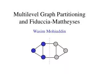
19. Multilevel Kernighan-Lin • Coarsen graph and expand partition using maximal matchings • Improve partition using Kernighan-Lin

20. Maximal Matching • Definition: A matching of a graph G(N,E) is a subset Em of E such that no two edges in Em share an endpoint • Definition: A maximal matching of a graph G(N,E) is a matching Em to which no more edges can be added and remain a matching • A simple greedy algorithm computes a maximal matching (recall section 9.2.1): Em= { } for i = 1 to |E| if i-th edge shares no endpoint with edges in Em, add i-th edge to Em end let Em be empty mark all nodes in N as unmatched for i = 1 to |N| … visit the nodes in any order if i has not been matched mark i as matched if there is an edge e=(i,j) where j is also unmatched, add e to Em mark j as matched endif endif endfor

21. Maximal Matching: Example

22. Example of Coarsening

23. Expanding a partition of Gc to a partition of G

24. Coordinate-Free: Spectral Bisection • Based on theory of Fiedler (1970s), popularized by Pothen, Simon, Liou (1990) • Motivation, by analogy to a vibrating string • Basic definitions • Vibrating string, revisited • Implementation using linear algebra

25. Motivation for Spectral Bisection • Vibrating string • Think of G = 1D mesh as masses (nodes) connected by springs (edges), i.e. a string that can vibrate • Vibrating string has modes of vibration, or harmonics • Label nodes by whether mode - or + to partition into N- and N+ • Same idea for other graphs (eg planar graph ~ trampoline)

26. 2nd eigenvector of L(planar mesh)

27. 4th eigenvector of L(planar mesh)

28. Details for Vibrating String Analogy: Recall F = ma • Force on mass j = k*[x(j-1) - x(j)] + k*[x(j+1) - x(j)] = -k*[-x(j-1) + 2*x(j) - x(j+1)] • F=ma yields m*x’’(j) = -k*[-x(j-1) + 2*x(j) - x(j+1)] (*) • Writing (*) for j=1,2,…,n yields x(1) x(1) - x(2) 1 -1 x(1) x(1) x(2) -x(1) + 2*x(2) - x(3) -1 2 -1 x(2) x(2) m * d2 … =-k* … =-k* … * … =-k*L* … dx2 x(j) -x(j-1) + 2*x(j) - x(j+1) -1 2 -1 x(j) x(j) … … … … … x(n) x(n-1) - x(n) -1 1 x(n) x(n) (-m/k) x’’ = L*x CS267 Lecture 23

29. Details for Vibrating String (continued) • -(m/k) x’’ = L*x, where x = [x1,x2,…,xn ]T • Seek solution of form x(t) = sin(a*t) * x0 • L * x0 = (m/k)*a2 * x0≡l * x0 • So l is an eigenvalue of L and x0 is its eigenvector • l determines frequency of vibration • x0 is its “shape” • L = 1 -1 called Laplacian of the graph -1 2 -1 (a 1D mesh in this example) …. -1 2 -1 -1 1

30. Laplacian Matrix of a Graph • Definition: The Laplacian matrix L(G) of a graph G(N,E) is an |N| by |N| symmetric matrix, with one row and column for each node. It is defined by • L(G) (i,i) = degree of node i (number of incident edges) • L(G) (i,j) = -1 if i ≠ j and there is an edge (i,j) • L(G) (i,j) = 0 otherwise

31. Example of L(G) for Simple Meshes

32. Properties of the Laplacian Matrix • The eigenvalues of L(G) are real and nonnegative: • 0 = l1l2  … ln • The number of connected components of G is equal to the number of li equal to 0. • Definition: l2 is the algebraic connectivity of G • The magnitude of l2 measures connectivity • In particular, l2≠ 0 if and only if G is connected. • Theorem (Fiedler, 75) The number of edges cut by any partitioning of G (including optimal one) is at least l2 * n / 4 • Spectral bisection algorithm to partition N = N- U N+ • Compute eigenvector v2 for l2 : L(G) * v2 = l2 * v2 • For each node n of G • if v2(n) < 0 put node n in N-, else put node n in N+ • Theorem (Fiedler): N- and N+ are connected (if no v2(n) = 0)

33. How do we compute v2 and l2 ? • Implementation via the Lanczos Algorithm • Approximation, requiring a number of matrix-vector multiplies by L • Studied in linear algebra classes • Have we made progress? • To optimize matrix-vector-multiply for a sparse matrix, we partition the graph of the matrix • To partition graph, we find an eigenvector of Laplacian matrix L associated with the graph • To find an eigenvector, we do matrix-vector-multiplies by L • Sounds like chicken and egg… • The first matrix-vector multiplies are slow, but we use them to learn how to make the rest faster • Useful when we want to do many sparse-matrix (or similar) operations • Useful when goal is partition itself (eg for image segmentation)

34. Multilevel Spectral Bisection • Coarsen graph and expand partition using maximal independent sets

35. Maximal Independent Sets • Definition: An independent set of a graph G(N,E) is a subset Ni of N such that no two nodes in Ni are connected by an edge • Definition: A maximal independent set of a graph G(N,E) is an independent set Ni to which no more nodes can be added and remain an independent set • A simple greedy algorithm computes a maximal independent set: let Ni be empty for k = 1 to |N| … visit the nodes in any order if node k is not adjacent to any node already in Ni add k to Ni endif endfor

36. Example of Coarsening - encloses domain Dk = node of Nc

37. Expanding a partition of Gc to a partition of G • Need to convert an eigenvector vc of L(Gc) to an approximate eigenvector v of L(G) • Use interpolation: For each node j in N ifj is also a node in Nc, then v(j) = vc(j) … use same eigenvector component else v(j) = average of vc(k) for all neighbors k of j in Nc end if endif

38. Example: 1D mesh of 9 nodes

39. Available Software Implementations • Multilevel Kernighan/Lin • METIS (www.cs.umn.edu/~metis) • ParMETIS - parallel version • Multilevel Spectral Bisection • S. Barnard and H. Simon, “A fast multilevel implementation of recursive spectral bisection …”, Proc. 6th SIAM Conf. On Parallel Processing, 1993 • Chaco (www.cs.sandia.gov/CRF/papers_chaco.html) • Hybrids possible • Ex: Using Kernighan/Lin to improve a partition from spectral bisection • Recent package, collection of techniques • Zoltan (www.cs.sandia.gov/Zoltan)

40. Extra Slides

41. Comparison of methods • Compare only methods that use edges, not nodal coordinates • CS267 webpage and KK95a (see below) have other comparisons • Metrics • Speed of partitioning • Number of edge cuts • Other application dependent metrics • Summary • No one method best • Multi-level Kernighan/Lin fastest by far, comparable to Spectral in the number of edge cuts • www-users.cs.umn.edu/~karypis/metis/publications/main.html • see publications KK95a and KK95b • Spectral give much better cuts for some applications • Ex: image segmentation • See “Normalized Cuts and Image Segmentation” by J. Malik, J. Shi CS267 Lecture 8

42. Number of edges cut for a 64-way partition For Multilevel Kernighan/Lin, as implemented in METIS (see KK95a) Expected # cuts for 2D mesh 6427 2111 1190 11320 3326 4620 1746 8736 2252 4674 7579 Expected # cuts for 3D mesh 31805 7208 3357 67647 13215 20481 5595 47887 7856 20796 39623 # of Nodes 144649 15606 4960 448695 38744 74752 10672 267241 17758 76480 201142 # of Edges 1074393 45878 9462 3314611 993481 261120 209093 334931 54196 152002 1479989 # Edges cut for 64-way partition 88806 2965 675 194436 55753 11388 58784 1388 17894 4365 117997 Graph 144 4ELT ADD32 AUTO BBMAT FINAN512 LHR10 MAP1 MEMPLUS SHYY161 TORSO Description 3D FE Mesh 2D FE Mesh 32 bit adder 3D FE Mesh 2D Stiffness M. Lin. Prog. Chem. Eng. Highway Net. Memory circuit Navier-Stokes 3D FE Mesh Expected # cuts for 64-way partition of 2D mesh of n nodes n1/2 + 2*(n/2)1/2 + 4*(n/4)1/2 + … + 32*(n/32)1/2 ~ 17 * n1/2 Expected # cuts for 64-way partition of 3D mesh of n nodes = n2/3 + 2*(n/2)2/3 + 4*(n/4)2/3 + … + 32*(n/32)2/3 ~ 11.5 * n2/3 CS267 Lecture 8

43. Speed of 256-way partitioning (from KK95a) Partitioning time in seconds # of Nodes 144649 15606 4960 448695 38744 74752 10672 267241 17758 76480 201142 # of Edges 1074393 45878 9462 3314611 993481 261120 209093 334931 54196 152002 1479989 Multilevel Spectral Bisection 607.3 25.0 18.7 2214.2 474.2 311.0 142.6 850.2 117.9 130.0 1053.4 Multilevel Kernighan/ Lin 48.1 3.1 1.6 179.2 25.5 18.0 8.1 44.8 4.3 10.1 63.9 Graph 144 4ELT ADD32 AUTO BBMAT FINAN512 LHR10 MAP1 MEMPLUS SHYY161 TORSO Description 3D FE Mesh 2D FE Mesh 32 bit adder 3D FE Mesh 2D Stiffness M. Lin. Prog. Chem. Eng. Highway Net. Memory circuit Navier-Stokes 3D FE Mesh Kernighan/Lin much faster than Spectral Bisection! CS267 Lecture 8

44. Beyond Simple Graph Partitioning • Undirected graphs model symmetric matrices, not unsymmetric ones • More general graph models include: • Hypergraph: nodes are computation, edges are communication, but connected to a set (>= 2) of nodes • HMETIS package • Bipartite model: use bipartite graph for directed graph • Multi-object, Multi-Constraint model: use when single structure may involve multiple computations with differing costs • For more see Bruce Hendrickson’s web page • www.cs.sandia.gov/~bahendr/partitioning.html • “Load Balancing Myths, Fictions & Legends” CS267 Lecture 8

45. Coordinate-Free Partitioning: Summary • Several techniques for partitioning without coordinates • Breadth-First Search – simple, but not great partition • Kernighan-Lin – good corrector given reasonable partition • Spectral Method – good partitions, but slow • Multilevel methods • Used to speed up problems that are too large/slow • Coarsen, partition, expand, improve • Can be used with K-L and Spectral methods and others • Speed/quality • For load balancing of grids, multi-level K-L probably best • For other partitioning problems (vision, clustering, etc.) spectral may be better • Good software available CS267 Lecture 13

46. Is Graph Partitioning a Solved Problem? • Myths of partitioning due to Bruce Hendrickson • Edge cut = communication cost • Simple graphs are sufficient • Edge cut is the right metric • Existing tools solve the problem • Key is finding the right partition • Graph partitioning is a solved problem • Slides and myths based on Bruce Hendrickson’s: “Load Balancing Myths, Fictions & Legends” CS267 Lecture 13

47. Myth 1: Edge Cut = Communication Cost • Myth1: The edge-cut deceit edge-cut = communication cost • Not quite true: • #vertices on boundary is actual communication volume • Do not communicate same node value twice • Cost of communication depends on # of messages too (a term) • Congestion may also affect communication cost • Why is this OK for most applications? • Mesh-based problems match the model: cost is ~ edge cuts • Other problems (data mining, etc.) do not CS267 Lecture 13

48. Myth 2: Simple Graphs are Sufficient • Graphs often used to encode data dependencies • Do X before doing Y • Graph partitioning determines data partitioning • Assumes graph nodes can be evaluated in parallel • Communication on edges can also be done in parallel • Only dependence is between sweeps over the graph • More general graph models include: • Hypergraph: nodes are computation, edges are communication, but connected to a set (>= 2) of nodes • Bipartite model: use bipartite graph for directed graph • Multi-object, Multi-Constraint model: use when single structure may involve multiple computations with differing costs CS267 Lecture 13

49. Myth 3: Partition Quality is Paramount • When structure are changing dynamically during a simulation, need to partition dynamically • Speed may be more important than quality • Partitioner must run fast in parallel • Partition should be incremental • Change minimally relative to prior one • Must not use too much memory • Example from Touheed, Selwood, Jimack and Bersins • 1 M elements with adaptive refinement on SGI Origin • Timing data for different partitioning algorithms: • Repartition time from 3.0 to 15.2 secs • Migration time : 17.8 to 37.8 secs • Solve time: 2.54 to 3.11 secs CS267 Lecture 13

50. References • Details of all proofs on Jim Demmel’s 267 web page • A. Pothen, H. Simon, K.-P. Liou, “Partitioning sparse matrices with eigenvectors of graphs”, SIAM J. Mat. Anal. Appl. 11:430-452 (1990) • M. Fiedler, “Algebraic Connectivity of Graphs”, Czech. Math. J., 23:298-305 (1973) • M. Fiedler, Czech. Math. J., 25:619-637 (1975) • B. Parlett, “The Symmetric Eigenproblem”, Prentice-Hall, 1980 • www.cs.berkeley.edu/~ruhe/lantplht/lantplht.html • www.netlib.org/laso CS267 Lecture 13